Whitebox QGIS Practice 26 — Elevation Statistics of Two Basins: Means of 2,000.1 m and 1,924.3 m, a 76 m Gap
In practice 25 I subtracted basin B from the whole basin of outlet A and made an interval basin (A−B) polygon. The areas were already known: 121.878 ha and 21.1372 ha. This time I wanted to see how the two basins differ in terrain. Both drain to outlets near the same confluence, but one takes in a wide stretch of the upper main stream and the other is a short tributary. On the hillshade the interval basin seems to reach higher ridges, but to say that with numbers you need zonal statistics: the mean, median, minimum and maximum elevation of the DTM cells that fall inside each polygon.
I kept the method simple. Merge the two polygons into one layer, run QGIS Zonal statistics once, and compare the results in one table. Then compute the same statistics again using the practice 22 Watershed raster as zones (value 1 = A's share, value 2 = B), to check that the polygon route and the raster route count the same cells. The two routes matched down to the cell count, and the interval basin was about 76 m higher on average.
Data
The statistics are computed on the 1 m DTM from practice 11 (USGS 3DEP tile 13SDE474426, EPSG:26913, built from ground points). The polygons and the zone raster are outputs of earlier practices, copied into a new input folder; the copies have the same hashes as the originals.
| Input | Original source | Content |
|---|---|---|
| wb26_input_dtm1m.tif | Practice 11 DTM | 1500×1500 cells, 1 m, float32, NoData −32768 |
| wb26_input_interval_A_minus_B.shp | Practice 25 wb25_interval_area | Interval basin 1,218,780 m², valid polygon (one 7 m² hole), VALUE 1 |
| wb26_input_poly_B.shp | Practice 24 wb24_poly_ab_1 | Basin B 211,372 m², valid polygon, VALUE 2 |
| wb26_input_watershed_ab_wb22.tif | Practice 22 Watershed (A, B order) | Value 1: 1,218,780 cells, value 2: 211,372 cells, same grid as the DTM |
The whole DTM has 1,834 NoData cells, but none fall inside the two basins. So the cell counts below equal the polygon areas in m².
Merging the two polygons into one layer
I opened Processing Toolbox → Vector general → Merge vector layers. You could run zonal statistics on each layer separately, but then the results end up in two files that you have to combine again to compare. Making one layer from the start makes the table easier to read.
| Field | Value | Why |
|---|---|---|
| Input layers | Interval basin A minus B (practice 25), Basin B polygon (practice 24) | The two basins to compare |
| Destination CRS | Left empty | Both layers are EPSG:26913, so there is nothing to reproject |
| Add source layer information | Checked (default) | Adds layer and path fields, so you can tell which file each row came from |
| Merged | wb26_basins_merged.shp |
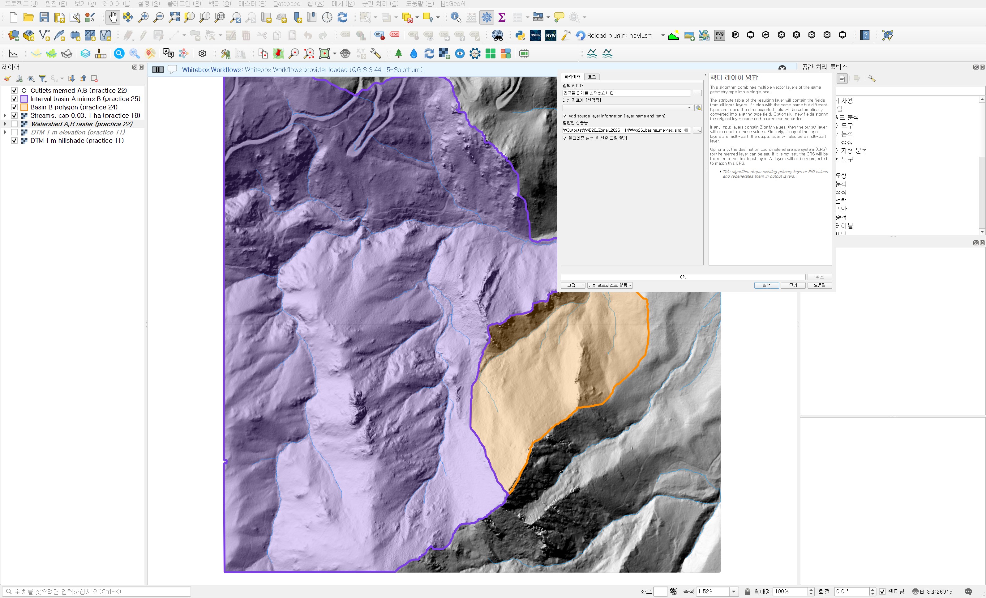
The merge produced two polygons, both valid. One thing in the attributes needs attention. Both source files have FID 1, so after the merge both rows still have FID 1. Use VALUE (1, 2) or the layer field to tell them apart. Also, the area_ha field existed only in the interval basin, so the B row came in as NULL. Merging takes the union of the fields; it does not fill in missing values.
Zonal statistics
I used Processing Toolbox → Raster analysis → Zonal statistics. This is the version that writes the result to a new layer, so no fields are added to the source polygons.
| Field | Value | Why |
|---|---|---|
| Input layer | Basins merged (interval + B) | The layer just merged |
| Raster layer | DTM 1 m elevation (practice 11) | I loaded the same file a second time for the statistics, separate from the copy shown as a hillshade. The result is identical; it just avoids confusion in the layer list |
| Raster band | Band 1 | Single band |
| Output column prefix | z_ | Shapefile field names are cut at 10 characters, so keep it short; z_median and z_stdev still fit |
| Statistics to calculate | Count, Mean, Median, St dev, Minimum, Maximum, Range | Sum is meaningless for elevation, so I left it out. Count is there to check the area |
| Zonal statistics | wb26_zonal_dtm.shp |
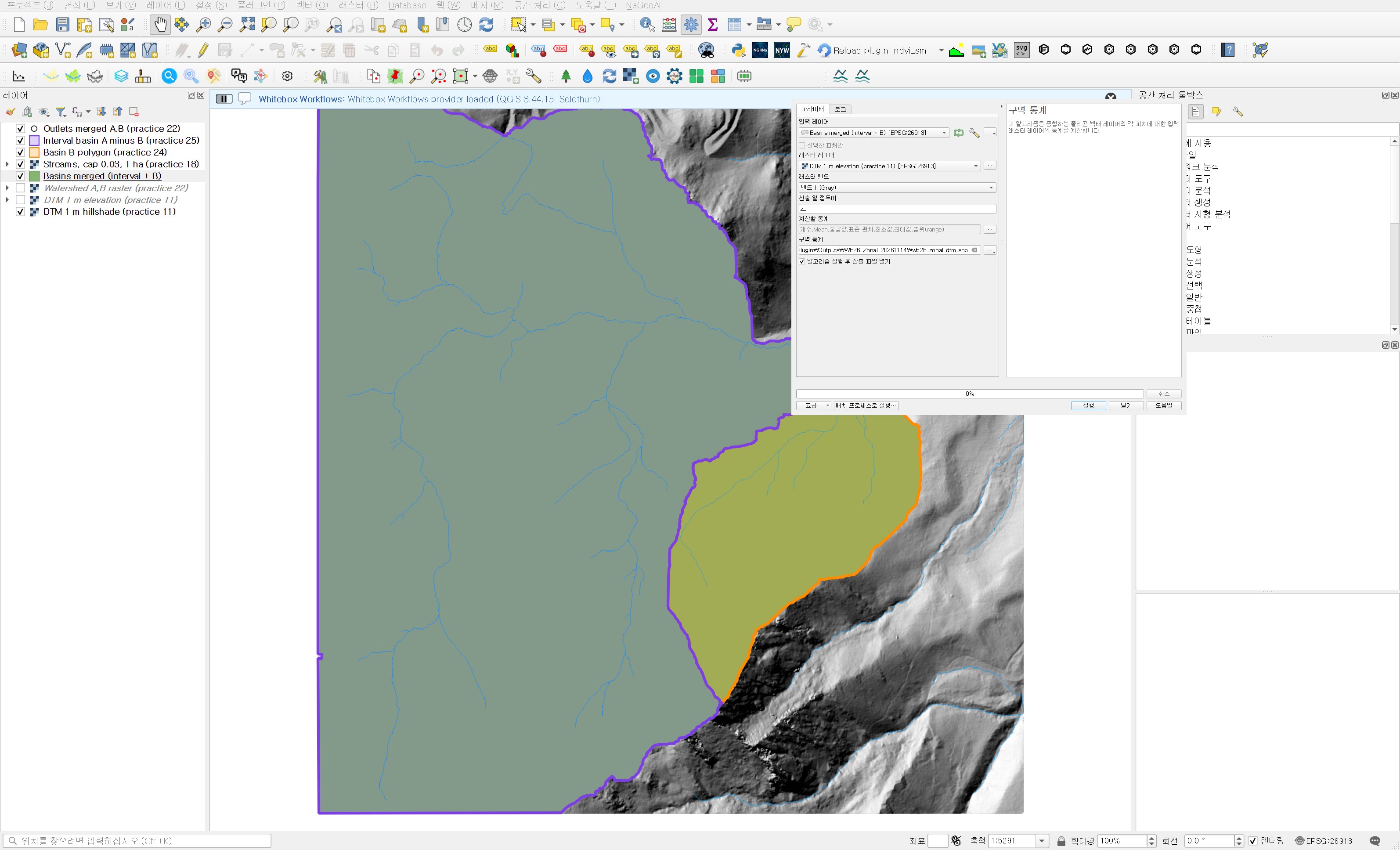
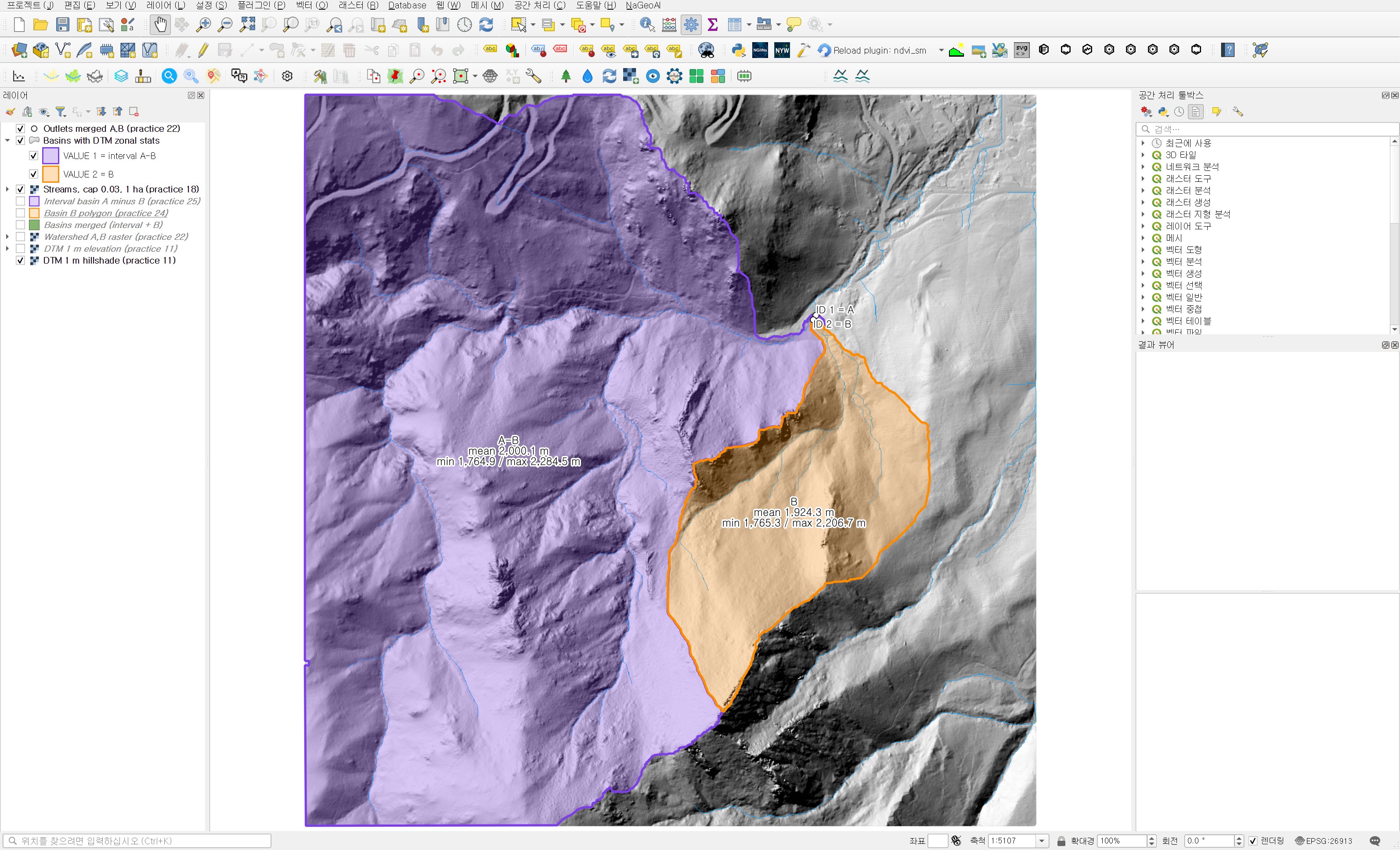
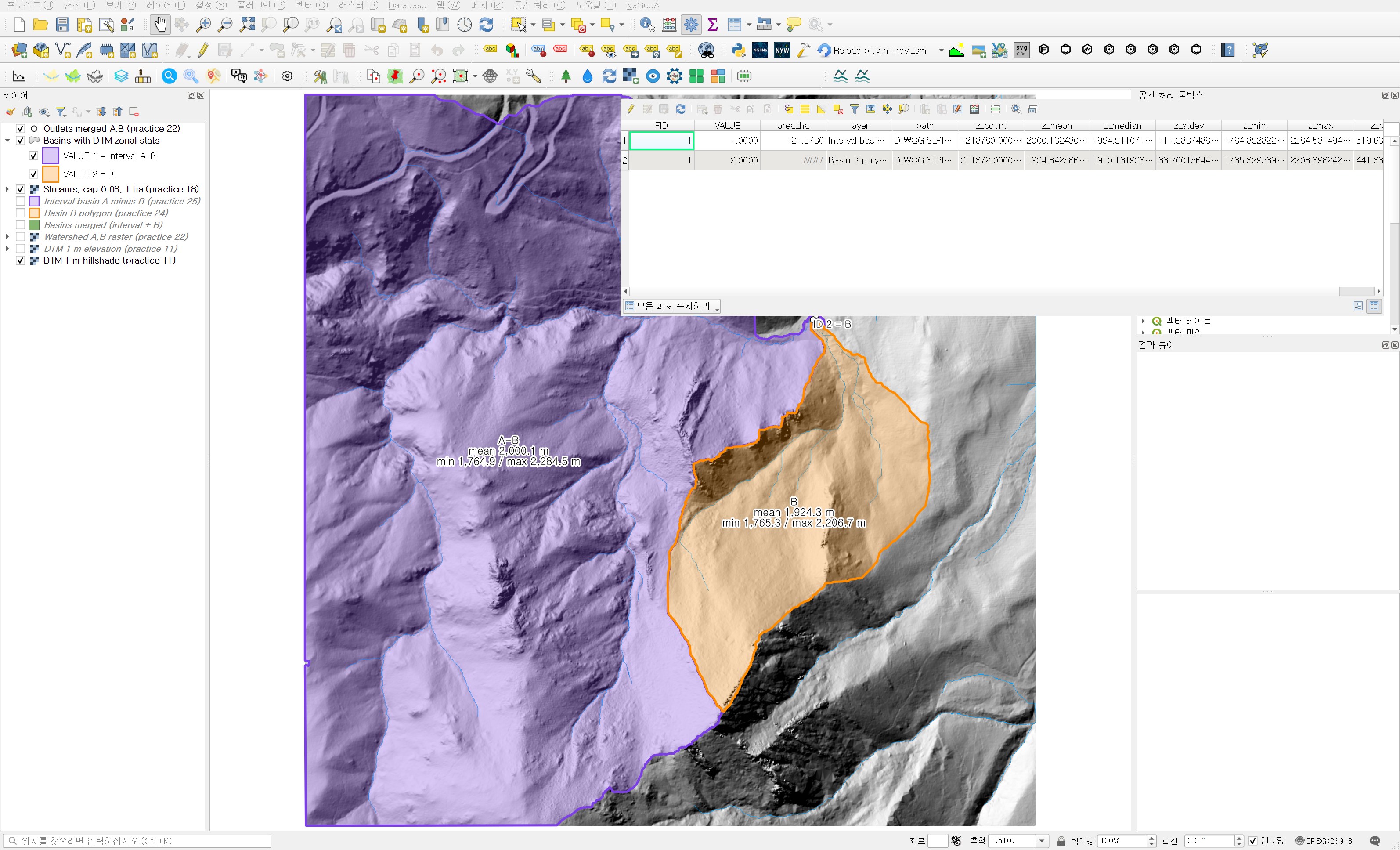
The run took less than a second. Counting about 1.5 million cells into two polygons is light work even for a 1 m DTM. I colored the result layer by VALUE and labeled it with the mean, minimum and maximum elevation.
The two basins in one table
| Item | Interval basin A−B (VALUE 1) | Basin B (VALUE 2) | Difference (A−B minus B) |
|---|---|---|---|
| Cell count (= area in m²) | 1,218,780 | 211,372 | |
| Mean elevation | 2,000.13 m | 1,924.34 m | +75.79 m |
| Median | 1,994.91 m | 1,910.16 m | +84.75 m |
| Minimum | 1,764.89 m | 1,765.33 m | −0.44 m |
| Maximum | 2,284.53 m | 2,206.70 m | +77.83 m |
| Range | 519.64 m | 441.37 m | +78.27 m |
| Standard deviation | 111.38 m | 86.70 m | +24.68 m |
The minimum elevations differ by only 0.44 m. In practice 22 outlets A and B were placed near the same confluence, so this is expected, and the number actually confirms that the outlets are in the right place. The difference is at the top. The maximum is almost 78 m higher, and the mean and median are 76–85 m higher. The impression that the interval basin collects water from higher ridges holds up in numbers.
The mean alone hides something, so I looked a little further at the distribution in the validation script. In the interval basin, 48.7% of cells are at or above 2,000 m and 8.4% are below 1,850 m. In B, 19.2% are at or above 2,000 m and 21.5% are below 1,850 m. The interquartile range is 1,910.80–2,087.21 m for the interval basin and 1,857.31–1,979.13 m for B, so B has a larger share of low ground near the outlet. B's median (1,910.16 m) being about 14 m below its mean (1,924.34 m) tells the same story: a long tail toward higher ground, with the bulk of the basin low.
The interval basin has the larger standard deviation. It is more than five times larger and spans a wider elevation range, so that is natural. A large standard deviation does not mean steep slopes, though. A large basin can have a wide elevation spread even if it is gentle; to talk about slope you need separate statistics on a slope raster.
Once more with raster zones
To check that the polygon route counted correctly, I ran Processing Toolbox → Raster analysis → Raster layer zonal statistics. This tool takes the zones as raster values instead of polygons, and the practice 22 Watershed raster is exactly such a zone raster.
| Field | Value | Why |
|---|---|---|
| Input layer | DTM 1 m elevation (practice 11) | The raster to summarize |
| Band number | 1 | |
| Zones layer | Watershed A,B raster (practice 22) | Value 1 = A's share, value 2 = B |
| Zones band number | 1 | |
| Reference layer | Input layer (default) | Both rasters share the same grid, so no resampling happens either way |
| Statistics | wb26_raster_zones_dtm.csv | A single table, so I saved it as CSV |
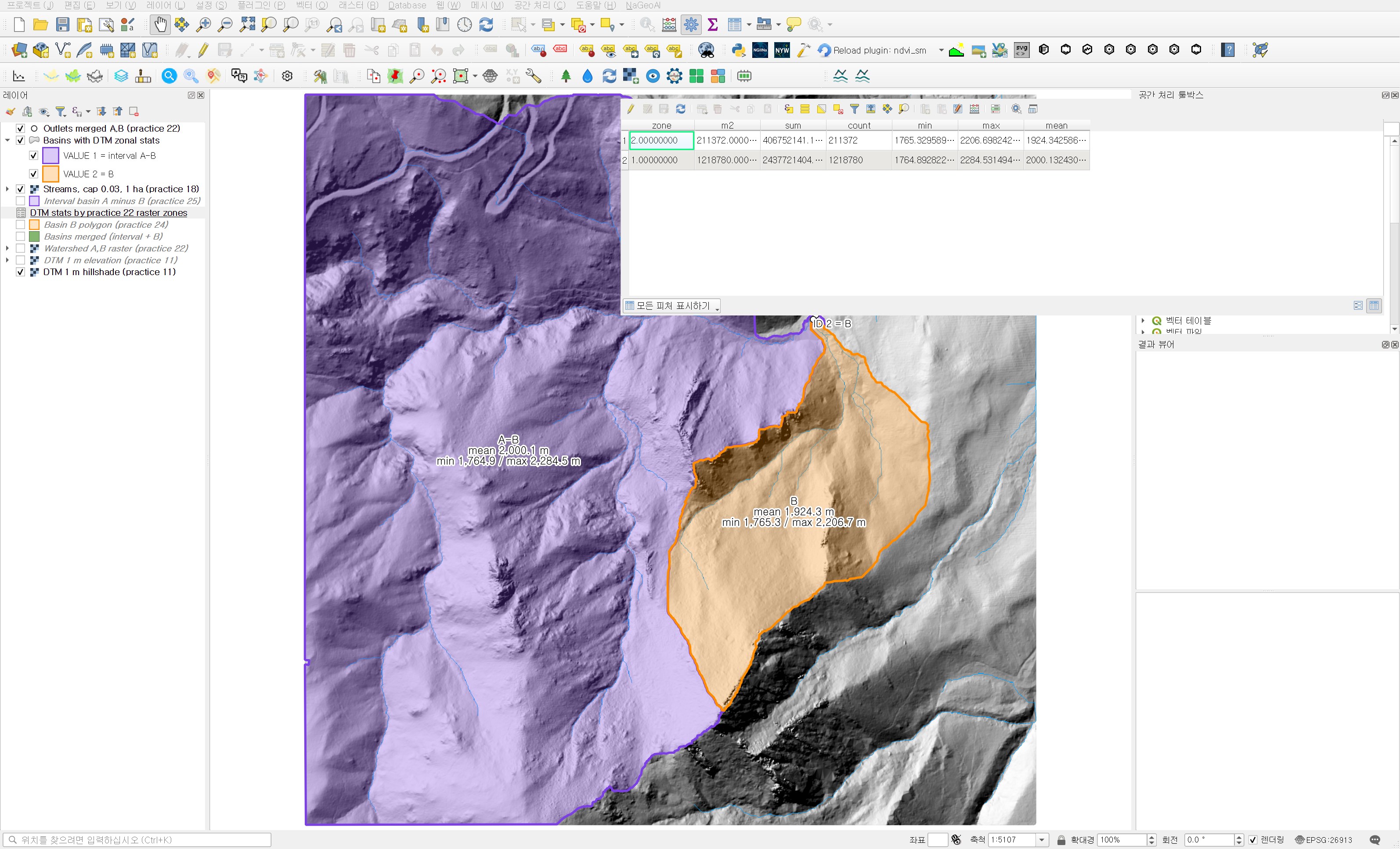
Zone 1 has 1,218,780 cells and zone 2 has 211,372, exactly the same counts as the polygon route. The mean, minimum and maximum match to the displayed digits. In the validation script I rasterized the polygons onto the same grid and compared them cell by cell with the practice 22 zones: 0 mismatched cells for both basins. This also means the 7 m² hole from practice 25 is excluded identically on both sides: in the polygon it is a hole, so no cell centers fall inside, and in the raster it was NoData to begin with.
This tool does not give the median or standard deviation; it adds sum and m2 (area) columns instead. So rather than one replacing the other, I think the two tools work best together: compute the statistics with one, and check the cell counts and means with the other.
Practical notes
- Zonal statistics counts only cells whose centers fall inside the polygon. When the polygon was made from the raster and follows cell edges, as here, the count and area match exactly. With boundaries from another source or a coarser raster, edge cells make count × cell area differ from the polygon area. Including the count and comparing it with the area shows such differences right away.
- Merging can leave duplicate FIDs from the sources. Check for a field that tells the rows apart (VALUE here), and create one before merging if there is none.
- When saving to shapefile, statistic field names are cut at 10 characters. Use a short prefix or save to GeoPackage.
- The same statistics on a DSM would mix in building and canopy heights. Use a bare-earth DTM to compare basin terrain; this data is a DTM built from ground points.
- Do not report only the difference in means; look at the median or quartiles too. In a basin like B, with most of its area on low ground, the mean is pulled above the typical elevation.
Next
The means and quartiles showed that the two basins have differently shaped elevation distributions. Next I plan to split the DTM into elevation bands (for example 50 m) and count the area in each band for each basin, to compare their elevation–area distributions side by side.
Work notes
This practice was run by a QGIS startup script that entered the values into the same dialogs, and the screenshots were captured at that time. The original project was left untouched and the work was done in a copy (QGIS_Play_NaGeoAI_20261114_26_zonal.qgz). The data source is USGS 3DEP (The National Map) tile 13SDE474426; the original DTM is not redistributed. The results were re-read by a separate script and the same statistics were computed independently with numpy (maximum difference below 1×10⁻¹² m), and the polygons were matched cell by cell against the practice 22 zone raster (0 mismatched cells). The quartiles and elevation-band shares come from that script. QGIS 3.44.15, GDAL 3.13.3. SHA-256 (first 12 characters):
- Input DTM 069a9c249240
- Input interval basin / B polygon .shp d891fa55042f / 0796f835c715
- Input Watershed (practice 22) 12c9fc71b969
- Merged .shp / .dbf 235891ed214a / 67d3965a6d72
- Zonal statistics .shp / .dbf 235891ed214a / e8e1b17ea680
- Raster zonal statistics .csv 0f55aa98e87c
This is an English adaptation of a post in the Korean Whitebox QGIS practice series. The original is here.
This post was drafted with the help of AI tools and reviewed by the author. Tool features and data portals change over time, so check the official documentation when you practice.

Comments
Post a Comment