Whitebox QGIS Practice 27 — Elevation-Area Distribution of Two Basins in 50 m Bands
In practice 26 I pulled elevation statistics for the interval basin (A−B) and basin B. The interval basin sat about 76 m higher on average, and B's median was about 14 m below its mean. Two means cannot tell you how much land lies at which elevation, and that distribution is what matters when you think about flood travel time, snow or vegetation zones. So this time I split the DTM into 50 m elevation bands, counted the band cells inside each basin, and put the two elevation-area distributions side by side.
Two built-in QGIS processing algorithms are enough. Reclassify by table turns elevation into band codes, and Zonal histogram counts the cells of each code inside the polygons. The DTM is 1 m, so one cell is 1 m² and a cell count is an area.
Data
I copied the practice 11 1 m DTM (USGS 3DEP tile 13SDE474426, EPSG:26913, a DTM built from ground points) and the merged polygon layer from practice 26 into a new input folder. The copies have the same hashes as the originals.
| Input | Source | Content |
|---|---|---|
| wb27_input_dtm1m.tif | Practice 11 DTM | 1500×1500 cells, 1 m, float32, NoData −32768 (1,834 cells), elevation 1,712.96 to 2,284.53 m |
| wb27_input_basins_merged.shp | Practice 26 wb26_basins_merged | VALUE 1 = interval basin 1,218,780 m², VALUE 2 = basin B 211,372 m² |
Reclassifying elevation into 50 m band codes
The DTM ranges from 1,712.96 m to 2,284.53 m, so I set twelve 50 m bands from 1,700 m to 2,300 m. Instead of serial numbers (1, 2, 3) each band code is its lower bound (1700, 1750, …, 2250). That way the histogram field names later become the elevation itself, such as h_1900, and the table reads without a separate lookup.
I opened Processing Toolbox → Raster analysis → Reclassify by table and entered the following.
| Field | Value | Why |
|---|---|---|
| Raster layer | DTM 1 m elevation (practice 11) | Raw elevation |
| Band number | Band 1 | |
| Reclassification table | 12 rows × 3 columns: min 1700 / max 1750 / value 1700, … , min 2250 / max 2300 / value 2250 | 50 m steps, value is the lower bound |
| Output NoData value | −9999 | NoData suited to an integer output |
| Range boundaries | min <= value < max | So a cell at exactly 2,000 m falls in the 2000–2050 band |
| Use NoData when no range matches value | Checked | Values outside the table do not stay as raw values |
| Output data type | Int16 | Codes go up to 2250, so Int16 is enough and the file is small |
| Reclassified raster | wb27_dtm_bands50m.tif |
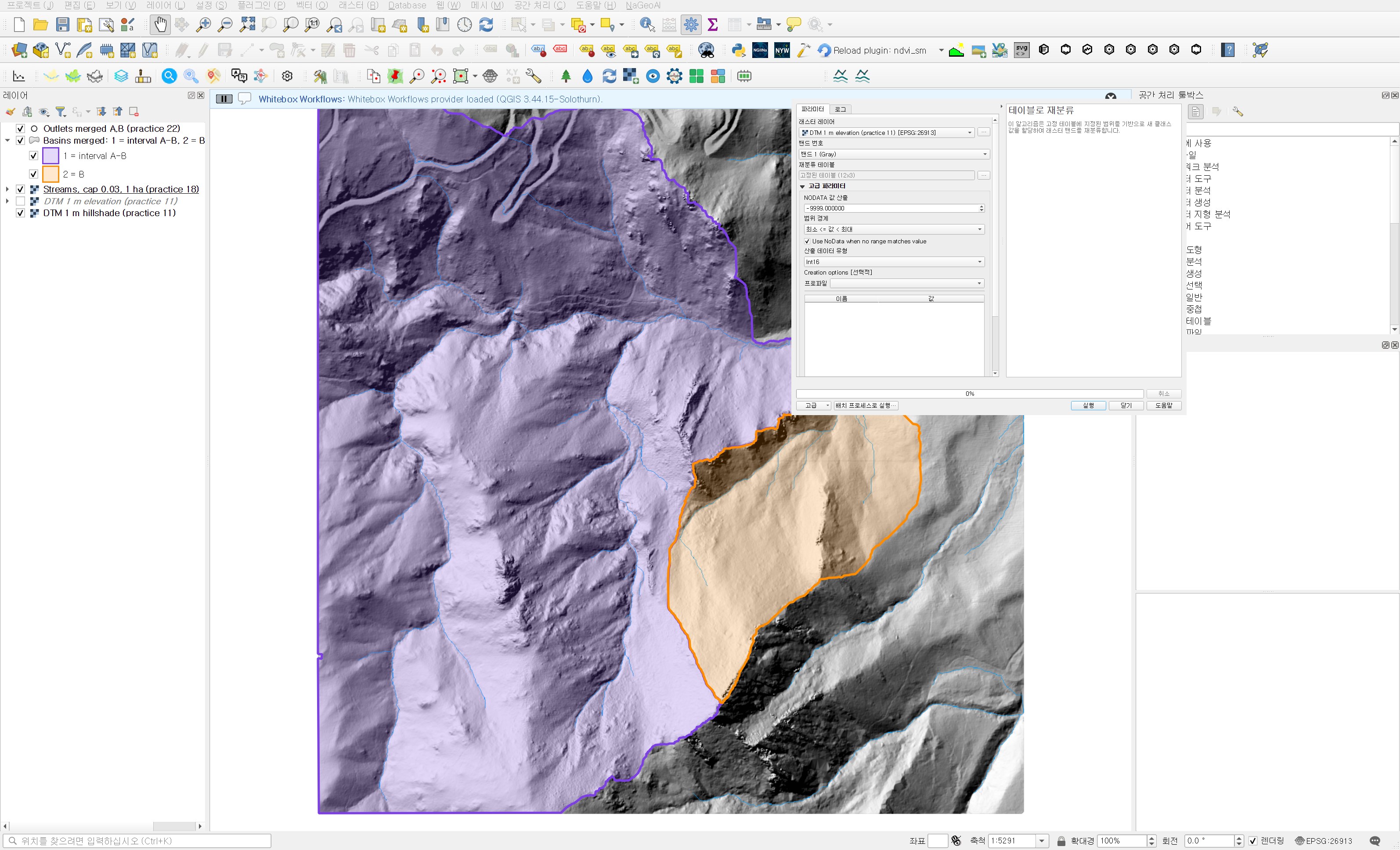
The default range boundary is "min < value <= max". With the default, a cell at exactly 2,000.0 m lands in the 1950–2000 band. Cells exactly on a boundary are rare in continuous float elevation, but if you are going to call a band "2000–2050 m", including the lower bound matches the name. The run took 0.13 seconds.
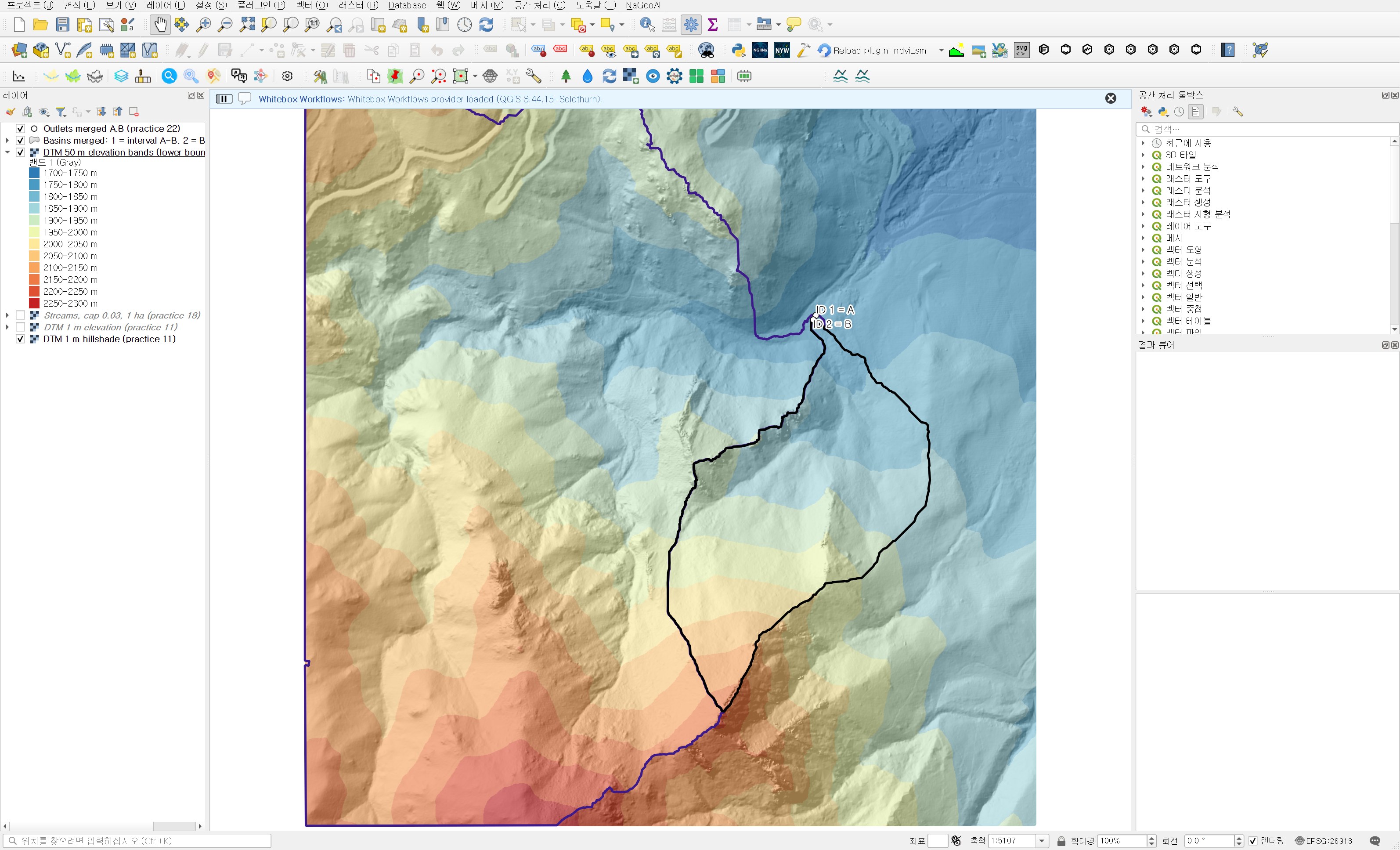
On the map, basin B sits mostly in the blue and light green bands and only its southern tip reaches orange. The interval basin covers nearly every colour, from blue near the outlet to the red ridges in the southwest. Time to check the numbers.
Counting cells per basin with Zonal histogram
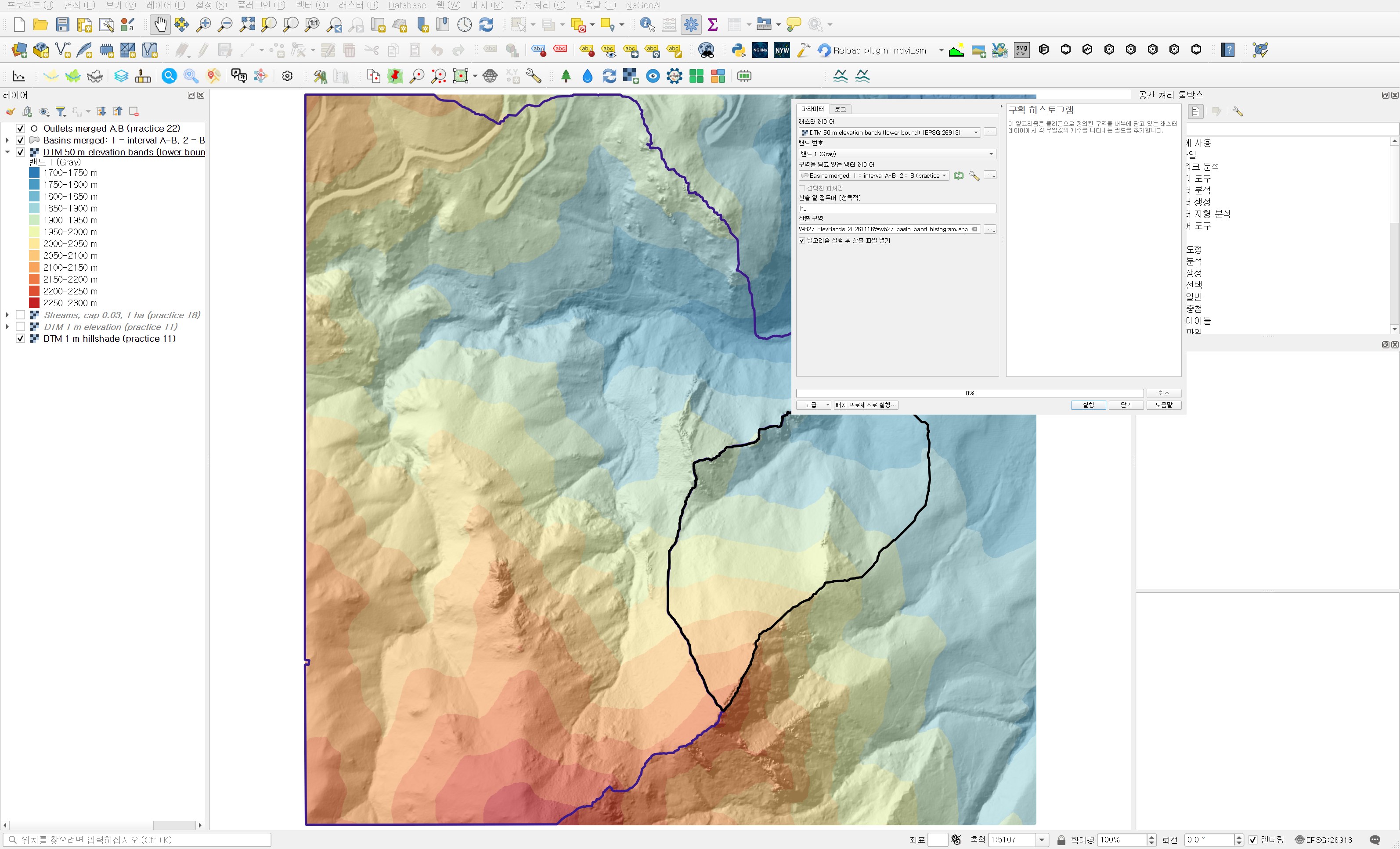
Processing Toolbox → Raster analysis → Zonal histogram adds one field per unique raster value to each polygon, holding the cell count. Where the zonal statistics of practice 26 give summary values such as mean and max, this tool gives a count table per value. It suits categorical rasters such as land cover, or band codes like these.
| Field | Value | Why |
|---|---|---|
| Raster layer | DTM 50 m elevation bands (lower bound) | The band codes just made |
| Band number | Band 1 | |
| Vector layer containing zones | Basins merged: 1 = interval A-B, 2 = B (practice 26) | Both basins in one layer give one result table |
| Output column prefix | h_ | h_2250 still fits the 10-character shapefile field limit |
| Output zones | wb27_basin_band_histogram.shp |
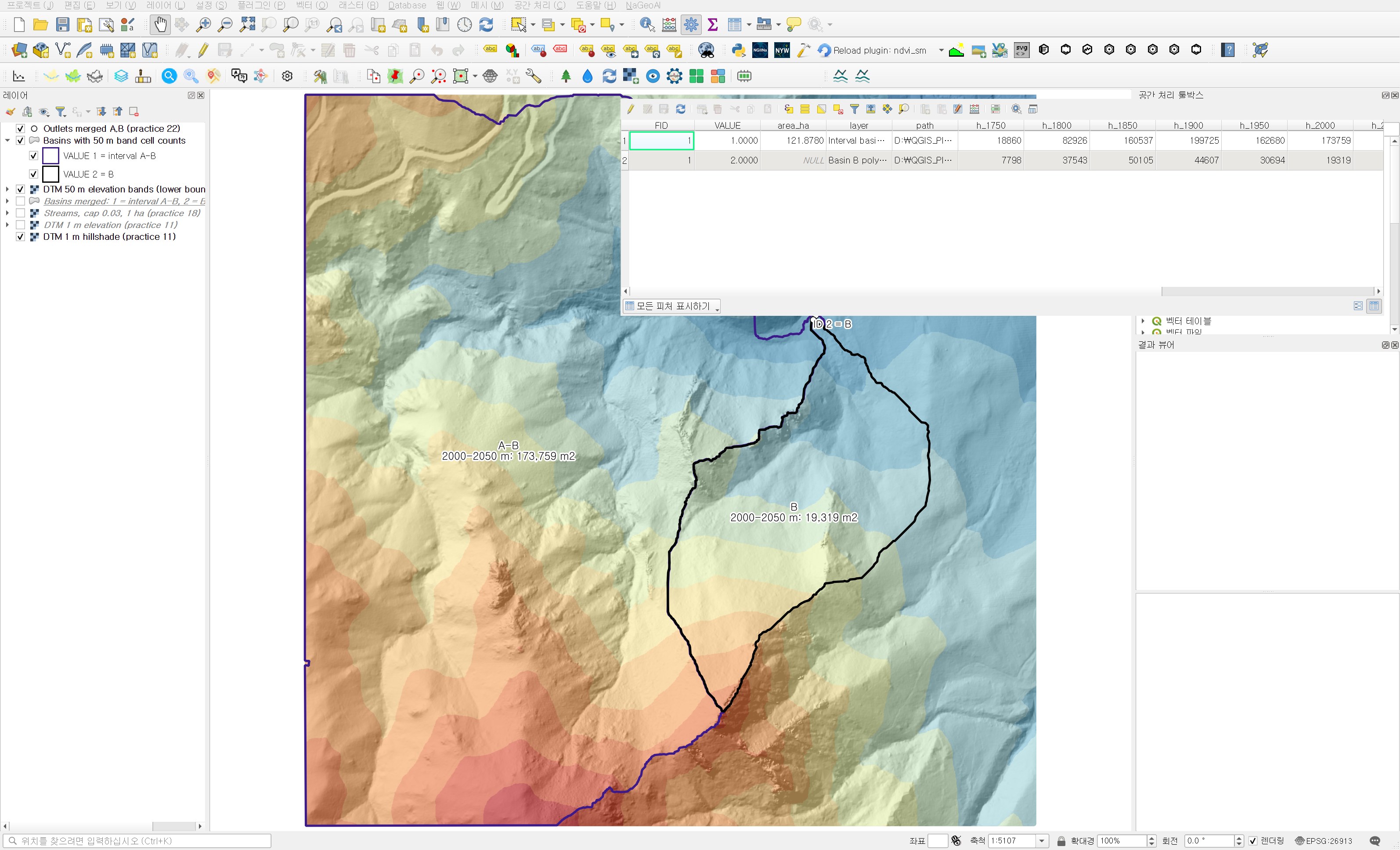
It ran in 0.28 seconds. The attribute table has 11 fields from h_1750 to h_2250. The 1700–1750 band has 89,224 cells in the whole DTM but none inside the two basins, so no field was created for it. That fits the basin minimums of 1,764.89 m and 1,765.33 m.
Area and share per band
I divided each count by the basin's total cell count. When one basin is more than five times larger than the other, shares compare better than absolute areas.
| Elevation band | Interval basin A−B area (m²) | Share | Basin B area (m²) | Share |
|---|---|---|---|---|
| 1750–1800 m | 18,860 | 1.55% | 7,798 | 3.69% |
| 1800–1850 m | 82,926 | 6.80% | 37,543 | 17.76% |
| 1850–1900 m | 160,537 | 13.17% | 50,105 | 23.71% |
| 1900–1950 m | 199,725 | 16.39% | 44,607 | 21.10% |
| 1950–2000 m | 162,680 | 13.35% | 30,694 | 14.52% |
| 2000–2050 m | 173,759 | 14.26% | 19,319 | 9.14% |
| 2050–2100 m | 153,334 | 12.58% | 11,747 | 5.56% |
| 2100–2150 m | 147,376 | 12.09% | 7,605 | 3.60% |
| 2150–2200 m | 74,906 | 6.15% | 1,913 | 0.91% |
| 2200–2250 m | 33,309 | 2.73% | 41 | 0.02% |
| 2250–2300 m | 11,368 | 0.93% | 0 | 0% |
| Total | 1,218,780 | 100% | 211,372 | 100% |
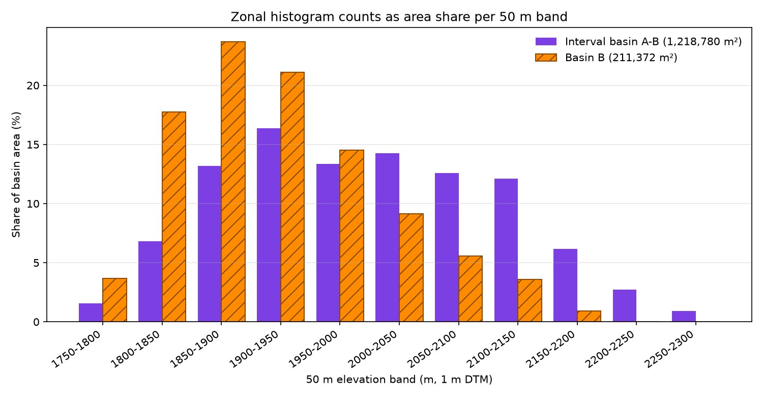
The two shapes are clearly different. Basin B is widest in the 1850–1900 m band at 23.71% and thins out quickly above it. The three bands from 1850 to 2000 m hold 59.33% of its area, and only 0.92% lies above 2150 m. Its bulk is in low ground not far from the outlet.
In the interval basin even the widest band (1900–1950 m) holds only 16.39%. Instead, the six bands from 1850 m to 2150 m each hold 12 to 16%, an almost flat run, and 9.81% lies above 2150 m. Its area is spread evenly across the whole elevation range. The "48.7% versus 19.2% above 2,000 m" from practice 26 now shows band by band.
This matters in practice because elevation ties to temperature, precipitation type and snow. Under the same storm, the interval basin with its larger share of high ground may receive snow over a wider area. This data alone cannot give snow cover or runoff timing, though. That needs a local temperature lapse rate or observed snow data. What is confirmed here is the elevation-area distribution.
Independent check
I recomputed the result in a separate script to see whether the reclassification followed the table and the histogram counted correctly. Dividing elevation by 50, flooring and multiplying by 50 in numpy gave the same band codes, with 0 differing cells across all 2.25 million cells. Rasterizing the polygons on the same grid by cell centre and counting per band also matched the attribute table in every band for both basins. The per-basin totals are 1,218,780 and 211,372, exactly the areas from practice 26.
Practical notes
- The default range boundary in Reclassify by table is "min < value <= max". If you name bands by their lower bound, switch to "min <= value < max".
- Check that the table covers the full DTM range. If "Use NoData when no range matches value" is off, out-of-range values stay as raw values and mix in like stray codes.
- Zonal histogram counts only cells whose centre is inside the polygon. With polygons made from the same raster, as here, counts and area match exactly. With boundaries from another source, edge cells make the total differ from the polygon area, so compare the two once.
- More bands mean more shapefile fields and a very wide attribute table. For a comparison table, export to CSV or convert to a share table as done here.
- The 50 m step was chosen to give about ten bands over this basin's elevation range of about 520 m. For a basin with a narrower range, use a smaller step to see the shape.
Next
With elevation covered, slope comes next. In practice 26 I noted that a large standard deviation does not mean steep terrain. Next I plan to derive a slope raster from the DTM and compare the slope distributions of the two basins the same way, with band reclassification and Zonal histogram.
Work notes
This session was run by a QGIS startup script that filled in the same dialogs and ran them, and the screens are captures from that run. The original project was left untouched and the work was done in a copy (QGIS_Play_NaGeoAI_20261116_27_elevbands.qgz). The data source is USGS 3DEP (The National Map) tile 13SDE474426, and the original DTM is not redistributed. Figure 5, the shares and the independent check come from a separate script that re-reads the output files. QGIS 3.44.15. First 12 characters of SHA-256:
- Input DTM 069a9c249240
- Input merged polygons .shp / .dbf 235891ed214a / 67d3965a6d72
- 50 m band raster 8ac146e8da50
- Zonal histogram .shp / .dbf 235891ed214a / bf5a73f6f6d7
This is an English adaptation of a post in the Korean Whitebox QGIS practice series. The original is here.
This post was drafted with the help of AI tools and reviewed by the author. Tool features and data portals change over time, so check the official documentation when you practice.


Comments
Post a Comment