Whitebox QGIS Practice 28 — Slope Distribution of Two Basins in 5° Classes
In practice 27 I split the two basins' elevation-area distribution into 50 m bands. The interval basin (A−B) had its area spread evenly from 1,850 m to 2,150 m, while basin B had its bulk between 1,850 and 2,000 m. With elevation distributions that different, it is easy to assume the slopes differ too. But a wide elevation range does not mean steep ground: a long, gentle hillside also covers a lot of elevation. So this time I derived a slope raster from the DTM and compared the two basins' slope distributions the same way as in practice 27, with band reclassification and a zonal histogram.
Slope comes from Whitebox Slope. The rest is two built-in QGIS algorithms, Reclassify by table and Zonal histogram. The DTM is 1 m, so one cell is 1 m² and a cell count is an area.
Data
I copied the same inputs as practice 27 into a new folder. The copies hash the same as the originals.
| Input | Original source | Content |
|---|---|---|
| wb28_input_dtm1m.tif | Practice 11 DTM | USGS 3DEP tile 13SDE474426, EPSG:26913, 1500×1500 cells, 1 m, 1,834 NoData cells |
| wb28_input_basins_merged.shp | Practice 26 merged polygons | VALUE 1 = interval basin 1,218,780 m², VALUE 2 = basin B 211,372 m² |
A slope raster with Whitebox Slope
I opened Processing Toolbox → WhiteboxTools → Geomorphometric Analysis → Slope. It has only four fields.
| Field | Value | Why |
|---|---|---|
| Input DEM File | DTM 1 m elevation (practice 11) | A DTM built from ground points. A DSM with building and tree heights would give spurious steep slopes |
| Z Conversion Factor | 1.0 | Horizontal (UTM, m) and vertical (m) units match |
| Units | degrees | Degrees are easier to read when splitting into 5° classes |
| Output File | wb28_slope_deg.tif |
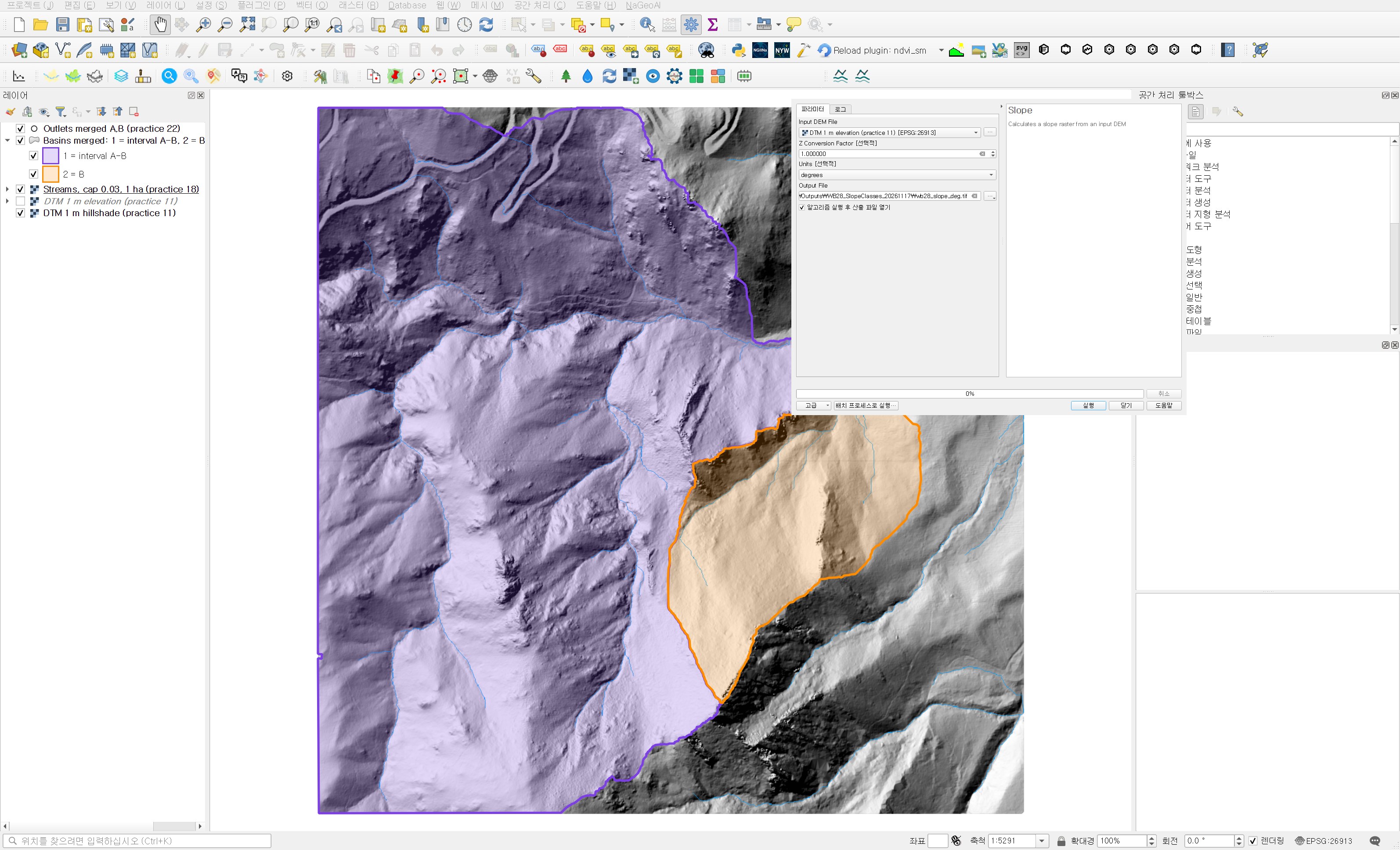
The Z conversion factor matters when you feed in a DEM in geographic coordinates. The horizontal unit is then degrees while elevation is in metres, and slopes come out close to zero. This DTM is projected, so 1.0 is right. The run finished in under a second. The output is float32 with 1,834 NoData cells, the same count as the DTM. Slopes range from 0.02° to 88.65°, with an overall median of 28.31° and a 99th percentile of 60.90°.
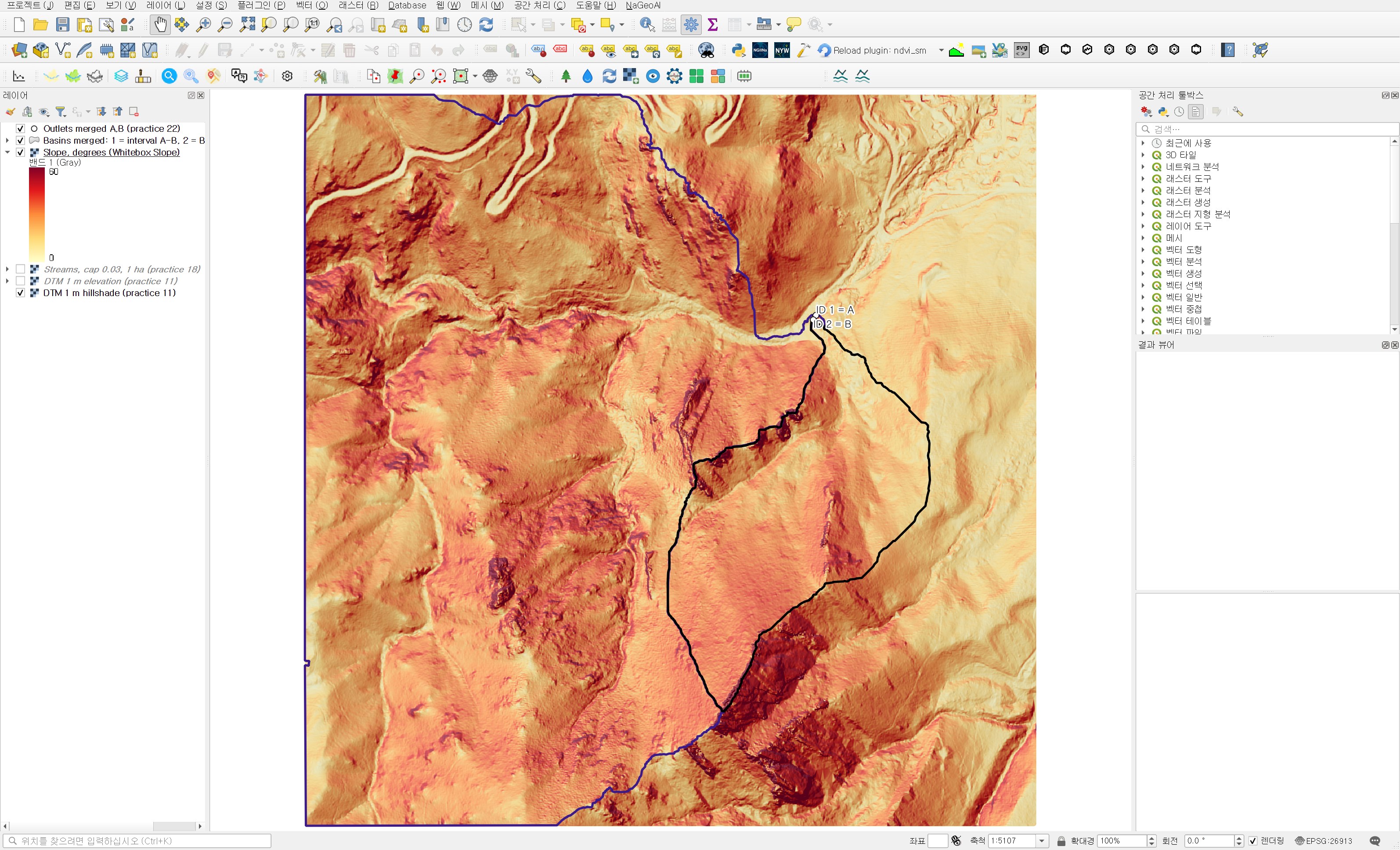
On the map the valley floor and the broad slope on the right are light, and the ridge slope at the southern end of basin B is the darkest. The places where the dark bands break up look like rock faces or stepped terrain. A continuous colour ramp shows where it is steep but not how much area is steep, so the next step is classes.
Reclassifying slope into 5° class codes
I made nine 5° classes from 0° to 45° and lumped everything at 45° and above into one, for ten classes in total. Slopes of 45° and above cover only about 6% of the area, so splitting them into 5° steps would give bars too low to compare. As in practice 27, the class code is the lower bound (0, 5, …, 45). That way the histogram fields are named after the angle, such as h_30, and the table reads directly.
| Field | Value | Why |
|---|---|---|
| Raster layer | Slope, degrees (Whitebox Slope) | The slope just created |
| Band number | Band 1 | |
| Reclassification table | 10 rows × 3 columns: min 0 / max 5 / value 0, … , min 40 / max 45 / value 40, min 45 / max 90 / value 45 | 5° steps, only the last is 45–90° |
| Output NoData value | −9999 | NoData that fits an integer output |
| Range boundaries | min <= value < max | So that a cell of exactly 30.0° falls in the 30–35° class |
| Use NoData when no range matches value | Checked | So values outside the table do not stay as they are |
| Output data type | Int16 | |
| Reclassified raster | wb28_slope_classes5deg.tif |
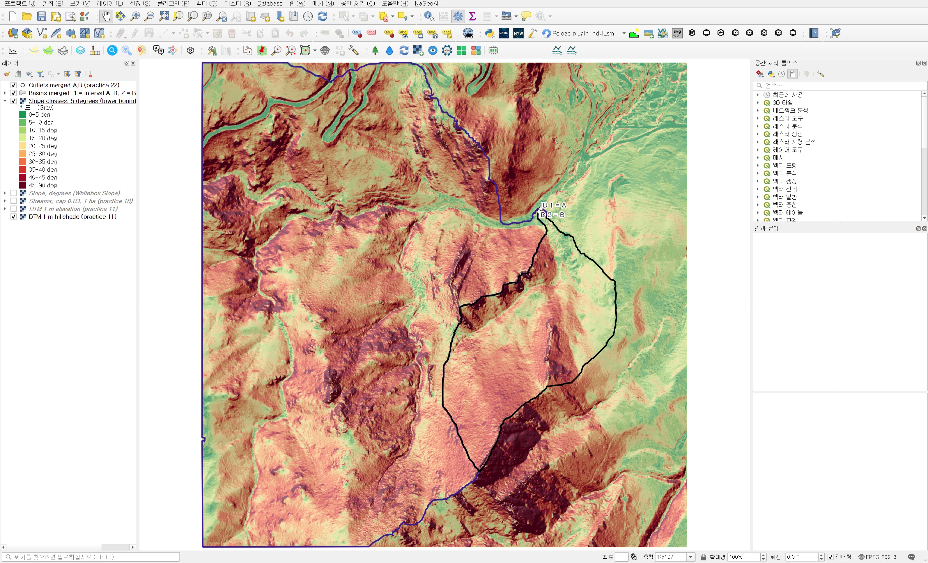
Across the whole DTM the largest class is 30–35° (443,952 cells), followed by 25–30° (416,238 cells). This is mountain terrain dominated by slopes of around 30°.
Counting cells per basin with Zonal histogram
| Field | Value | Why |
|---|---|---|
| Raster layer | Slope classes, 5 degrees (lower bound) | Class codes |
| Band number | Band 1 | |
| Vector layer containing zones | Basins merged: 1 = interval A-B, 2 = B (practice 26) | Both basins come out in one table |
| Output column prefix | h_ | h_0 to h_45 fit within the 10-character shapefile field limit |
| Output zones | wb28_basin_slope_histogram.shp |
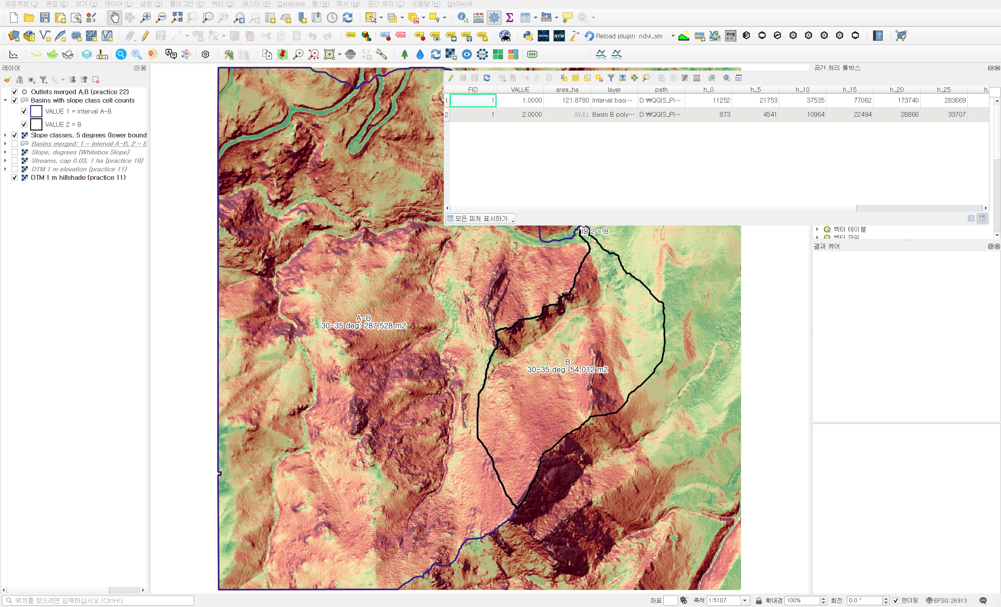
The run took under a second. All ten classes appear in both basins; even the 0–5° flat class shows up a little on the valley floor.
Area and share per class
| Slope class | Interval basin A−B area (m²) | Share | Basin B area (m²) | Share |
|---|---|---|---|---|
| 0–5° | 11,252 | 0.92% | 873 | 0.41% |
| 5–10° | 21,753 | 1.78% | 4,541 | 2.15% |
| 10–15° | 37,535 | 3.08% | 10,964 | 5.19% |
| 15–20° | 77,062 | 6.32% | 22,494 | 10.64% |
| 20–25° | 173,740 | 14.26% | 26,866 | 12.71% |
| 25–30° | 283,669 | 23.28% | 33,707 | 15.95% |
| 30–35° | 287,528 | 23.59% | 54,012 | 25.55% |
| 35–40° | 171,731 | 14.09% | 40,176 | 19.01% |
| 40–45° | 73,649 | 6.04% | 8,829 | 4.18% |
| 45–90° | 80,861 | 6.63% | 8,910 | 4.22% |
| Total | 1,218,780 | 100% | 211,372 | 100% |
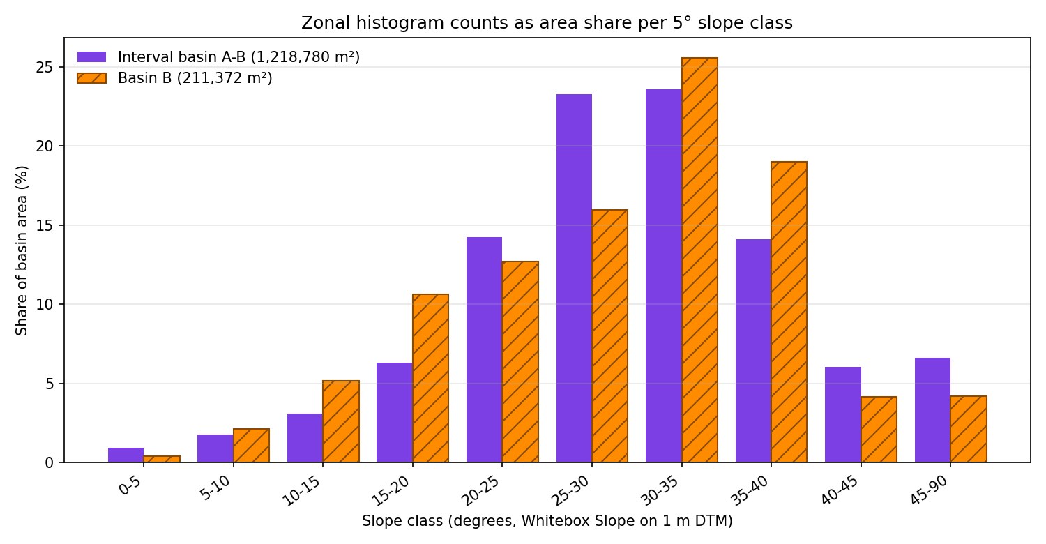
First, the summary values are almost the same. The median slope is 30.07° in the interval basin and 30.71° in B, and the largest class is 30–35° in both. The share at 30° and above is 50.36% against 52.95%, not much of a gap. Given how different the elevation distributions were in practice 27, that is a surprise. The guess that the interval basin, with its wider elevation range, would be steeper was wrong.
The difference is in the shape of the distribution. The interval basin has 61.12% of its area in the three classes from 20° to 35°, so it is thick in the middle. Its tail at 40° and above, however, is longer at 12.68%, against 8.39% in B. Basin B is the opposite and is wide at both ends. Gentle ground under 20° makes up 18.39% (12.11% in the interval basin), and steep 30–40° slopes make up 44.56% (37.68%). Gentle valley floor and 30-something slopes mix, with relatively little in the 20s between them. That gentle share is also why B's mean of 29.56° sits below its median.
In practice, how you read this depends on where you cut. If you report a "steep share" at 30°, the two basins are almost equal. Raise the cutoff to 40° and the interval basin has about 1.5 times as much. In landslide or rockfall screening, the threshold you choose can change the ranking. The threshold should come from the purpose of the review (guidelines, ground conditions), not from the data. Here I only checked the distribution.
Independent check
A separate script recomputed two things. First, it put the Whitebox slope values through the same table (lower bound included) with numpy, and the class codes differed from the QGIS reclassification in zero cells out of 2.25 million. Cell counts per class from rasterizing the polygons by cell centre matched the attribute table for every class in both basins, and the totals matched the practice 26 areas.
Second, it computed slope itself independently with a numpy Horn 3×3 method and compared. Over 2,242,172 cells, excluding the edges, the mean difference was 0.56° and 99% of cells were within 3.05°. 89.93% of cells fell in the same 5° class. Most cells agree, but on steep 1 m terrain some cells differ by several degrees. Whitebox Slope does not appear to compute slope exactly as Horn 3×3 does. If you compare across sessions or areas, it is safer to settle on one slope tool.
Things to watch in practice
- Compute slope from a DTM. On a DSM, building walls and canopy edges show up as steep slopes that have nothing to do with the terrain.
- For a DEM in geographic coordinates, project it first or set the Z conversion factor. Left as is, slopes are squashed toward 0°.
- If the last class is wide (45–90°), say so in the caption so readers do not read its bar height the same way as the others.
- Slope algorithms differ slightly between tools, so on the same DTM cells near a class boundary can land in different classes. Fix the tool and version for comparison work.
- If the Whitebox tools vanish from the toolbox and a yellow bar says the plugin was disabled because it previously crashed QGIS, QGIS turned off wbt_for_qgis at startup. That bar appeared in this run too, so I loaded the plugin for that session only. Before turning it back on in the Plugin Manager, find out what caused the crash.
Next session
With elevation and slope covered, aspect comes next. I plan to make an aspect raster with Whitebox Aspect, reclassify it into eight compass sectors, and compare which way the two basins' slopes face, using the same method.
Work notes
This session was run by a QGIS startup script that filled in the same dialogs and ran them, and the screens are captures from that run. The original project was left untouched and the work was done in a copy (QGIS_Play_NaGeoAI_20261117_28_slopebands.qgz). The data source is USGS 3DEP (The National Map) tile 13SDE474426, and the original DTM is not redistributed. Figure 5, the shares and the independent check come from a separate script that re-reads the output files. QGIS 3.44.15, with WhiteboxTools run through the wbt_for_qgis plugin. First 12 characters of SHA-256:
- Input DTM 069a9c249240
- Input merged polygons .shp / .dbf 235891ed214a / 67d3965a6d72
- Slope raster bdbbacc35eb1
- 5° class raster a01083bef248
- Zonal histogram .shp / .dbf 235891ed214a / 0880d61e7416
This is an English adaptation of a post in the Korean Whitebox QGIS practice series. The original is here.
This post was drafted with the help of AI tools and reviewed by the author. Tool features and data portals change over time, so check the official documentation when you practice.


Comments
Post a Comment