Whitebox QGIS Practice 29 — Aspect of Two Basins in Eight Directions, and a Z Factor That Flipped It by 180°
In sessions 27 and 28 I compared the elevation and slope of two basins with the same method: reclassify into bands, then count cells per basin with a zonal histogram. This time it is aspect, the direction a slope faces, measured clockwise from north toward the downhill side. 0° (360°) is north-facing, 90° east-facing, 180° south-facing. Sunlight, snowmelt timing, vegetation and soil moisture all follow aspect, so "which way do most slopes face" is often one of the first questions asked about a basin.
The steps are the same as in the last two sessions. Whitebox Aspect makes the aspect raster, Reclassify by table assigns eight compass codes, and Zonal histogram counts cells per basin. On the first run, however, the whole result came out rotated by 180°. Half of this post is about that.
Data
I copied the session 28 inputs into a new folder. The copied DTM has the same hash as the original.
| Input | Origin | Contents |
|---|---|---|
| wb29_input_dtm1m.tif | Session 11 DTM | USGS 3DEP tile 13SDE474426, EPSG:26913, 1500×1500 cells, 1 m, 1,834 NoData cells |
| wb29_input_basins_merged.shp | Session 26 merged polygons | VALUE 1 = interval basin (A−B) 1,218,780 m², VALUE 2 = basin B 211,372 m² |
First run: Z conversion factor set to 1.0
Processing Toolbox → WhiteboxTools → Geomorphometric Analysis → Aspect has only three fields. As with Slope in session 28, I entered 1.0 in Z Conversion Factor. The DTM is projected, with metres both horizontally and vertically, so 1.0 looked like the right value.
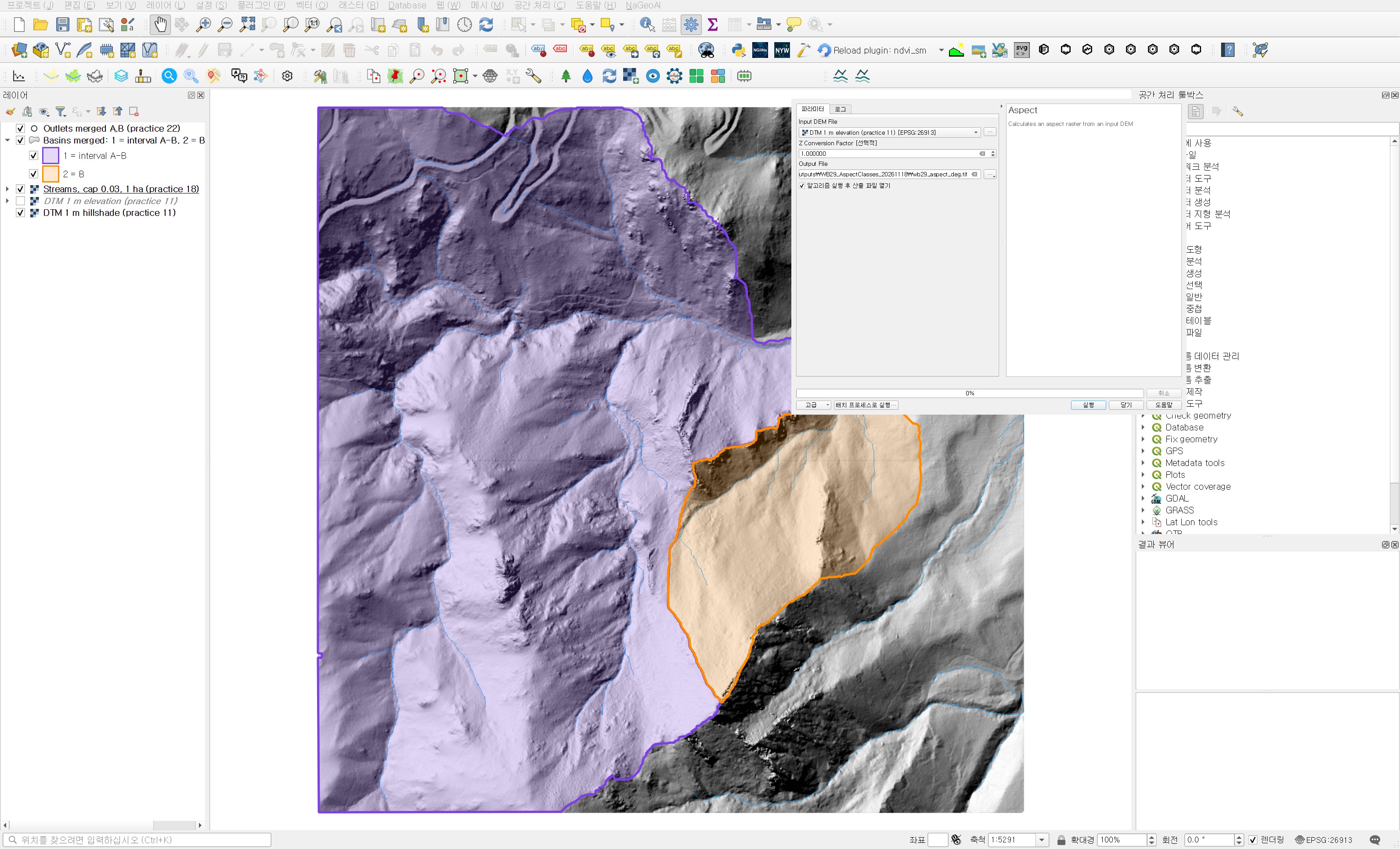
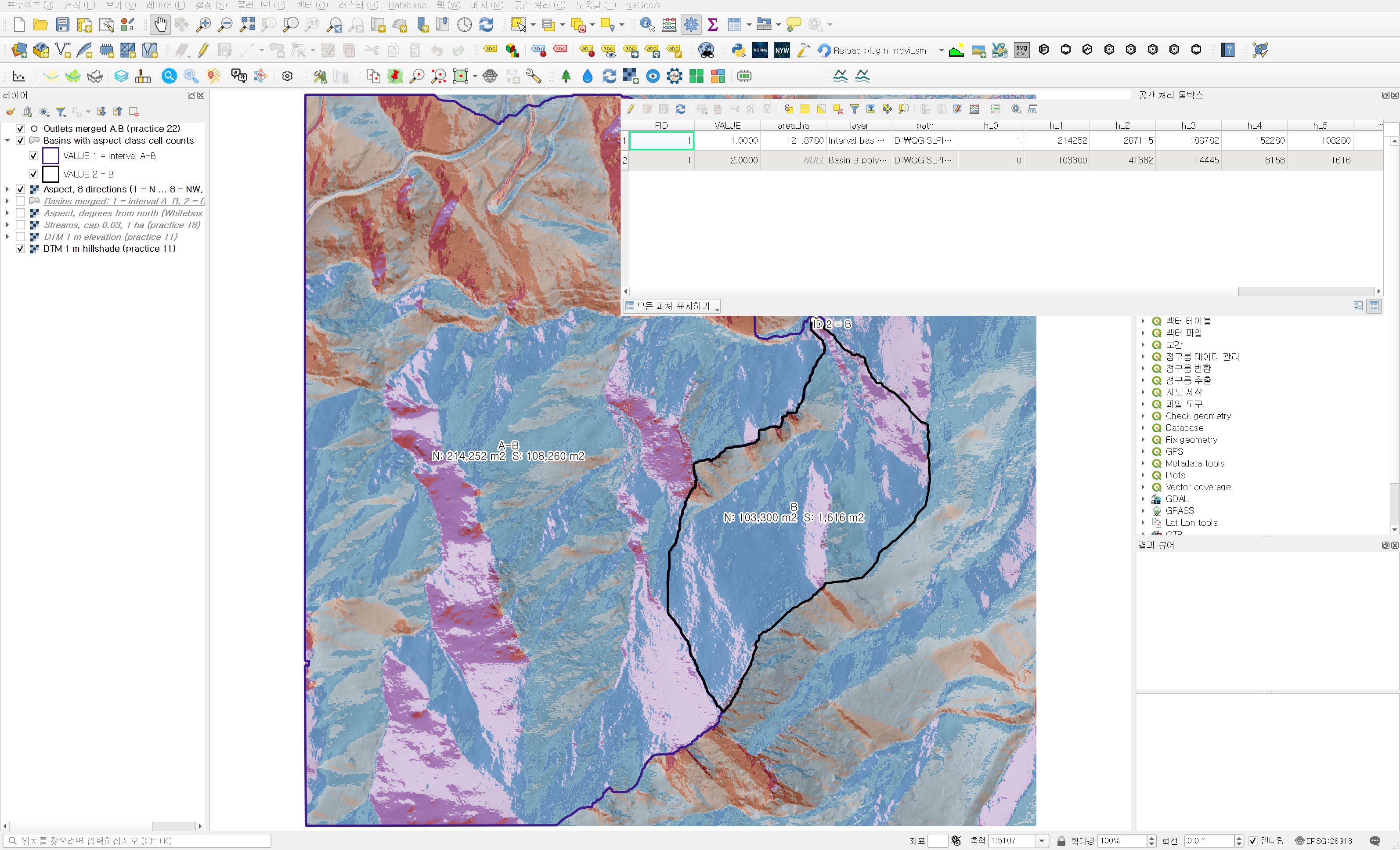
It finished in a few seconds with no error. After reclassifying into eight sectors, almost all of basin B came out in the south-facing colours (orange and red). The zonal histogram put 85.18% of basin B in SE, S and SW.
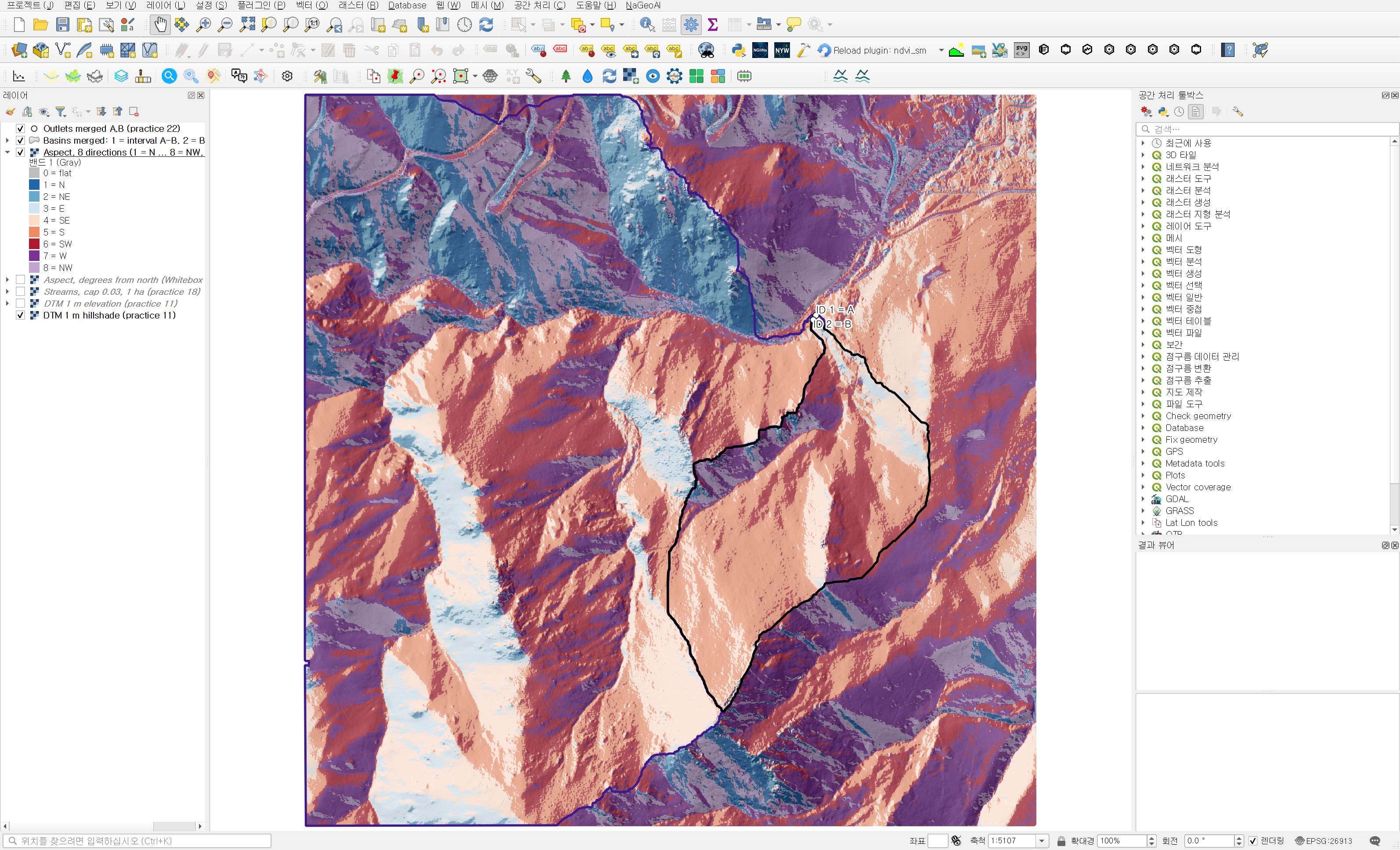
That did not look right. The outlet of basin B (ID 2 = B in the figure) is at the northern end of the basin. If water gathers at a northern outlet, the ground should generally drop toward the north, and north-facing slopes should dominate. Checking the DTM directly, the correlation between elevation and row number (which increases southward) inside basin B was 0.966. The south is high and the north is low. 85% south-facing does not fit that terrain.
Narrowing down the cause
I checked three things separately.
- Against the steepest-descent direction. I sampled 3,000 random DTM cells and found which of the eight neighbours drops most steeply. The Whitebox aspect was within 45° of that direction in 2 cells and off by 135° or more in 2,945.
- Against a numpy Horn 3×3 aspect. Compared with an independently computed aspect, the median difference was 179.0°. Not one sector but the whole raster was reversed.
- Running Whitebox directly. Outside QGIS, I ran Aspect with the same whitebox_tools.exe (v2.2.0) on the same DTM. Without a Z factor the sample cell came out at 91.36°; with
--zfactor=1.0it was 271.36°. The compression option and the number of threads did not change the result. On a synthetic plane rising to the north-east, which should face south-west (225°), I got 225° without the factor and 45° with 1.0.
So with this version, passing a Z conversion factor value to Aspect rotates the aspect by 180°. Comparing the first-run result with the final result below cell by cell, all 2,248,165 valid cells differ by exactly 180° (within 0.01°). I did not find out why the tool does this internally. I also set 1.0 for Slope in session 28, but slope is a magnitude with no direction, so it is not affected, and the mean difference from Horn 3×3 then was 0.56°.
Second run: leave the Z conversion factor empty
| Field | Value | Reason |
|---|---|---|
| Input DEM File | DTM 1 m elevation (practice 11) | Ground-point DTM. In a DSM, building walls and canopy edges scramble the aspect |
| Z Conversion Factor | Left empty (Not set) | It is optional. Entering a value reversed the aspect, as above |
| Output File | wb29_aspect_deg.tif | The first-run output was moved to a separate folder and kept |
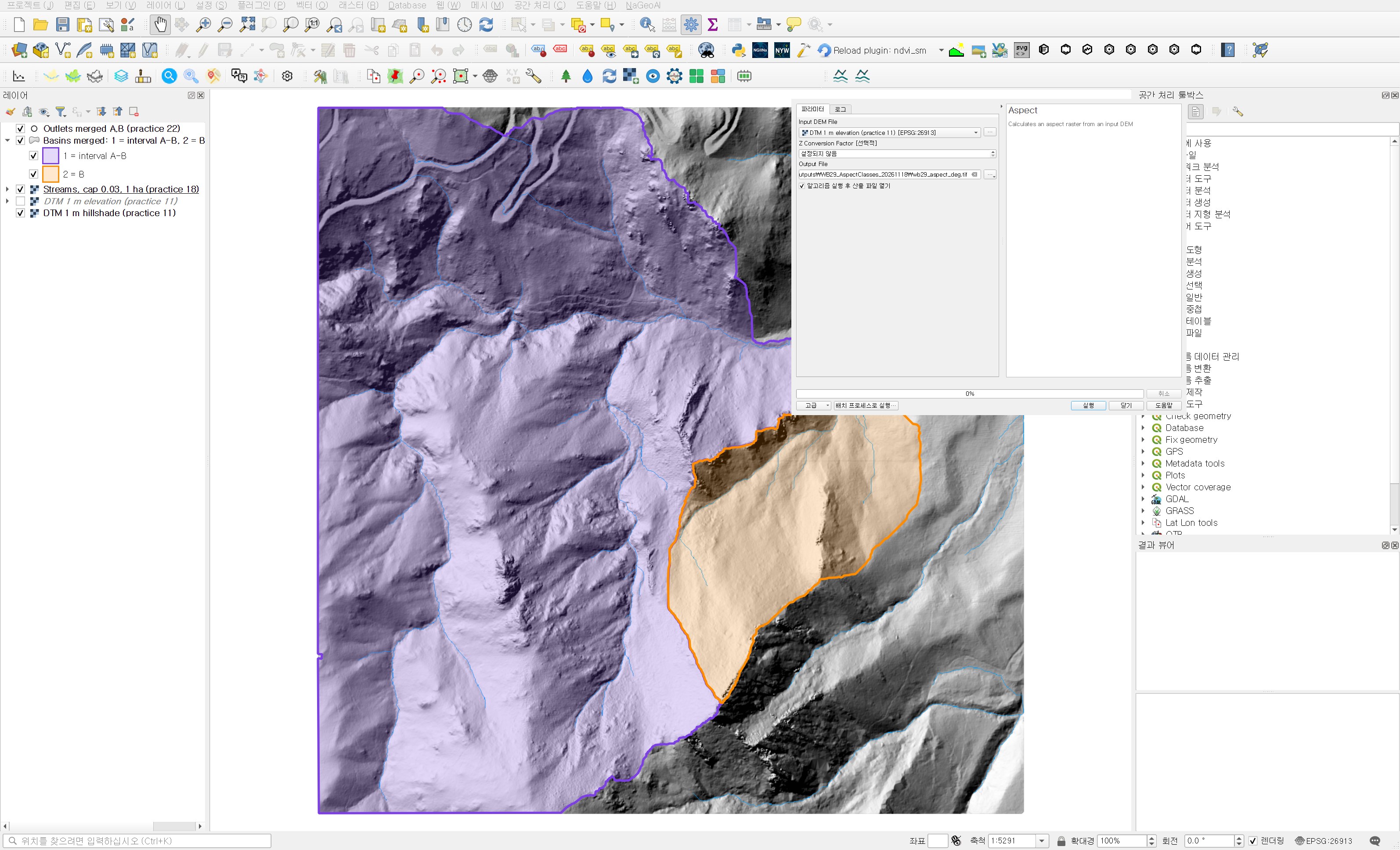
Run this way, --zfactor is dropped from the command line the plugin builds. The result is float32 with 1,834 NoData cells (same as the DTM) and values from 0.0002° to 359.9999°. Exactly one cell has the value −1. It appears to be the value Whitebox writes when it cannot assign a direction. In the synthetic-plane test, a plane tilted exactly north–south (zero east–west gradient) also came out as −1. Such cells are rare in natural terrain, but with data full of stepped, man-made surfaces it is worth counting the −1 cells once.
Reclassifying into eight sectors
I split aspect into eight 45° sectors. North straddles 0°, split into 337.5–360° and 0–22.5°, so both rows get code 1. Negative values (−1) go to a separate flat code 0. Codes run clockwise from 1 = N to 8 = NW, so the histogram fields h_1 to h_8 come out in compass order.
| Field | Value | Reason |
|---|---|---|
| Raster layer | Aspect, degrees from north (Whitebox Aspect) | The aspect just made |
| Band number | Band 1 | |
| Reclassification table | 10 rows: −1000–0 → 0, 0–22.5 → 1, 22.5–67.5 → 2, 67.5–112.5 → 3, 112.5–157.5 → 4, 157.5–202.5 → 5, 202.5–247.5 → 6, 247.5–292.5 → 7, 292.5–337.5 → 8, 337.5–361 → 1 | Two rows handle north crossing 0°. The last maximum is 361 so cells very close to 360° are not lost |
| Output no data value | −9999 | |
| Range boundaries | min <= value < max | A cell exactly on a boundary such as 22.5° goes to the next sector clockwise |
| Use no data when no range matches value | Checked | |
| Output data type | Int16 | |
| Reclassified raster | wb29_aspect_8dir.tif |
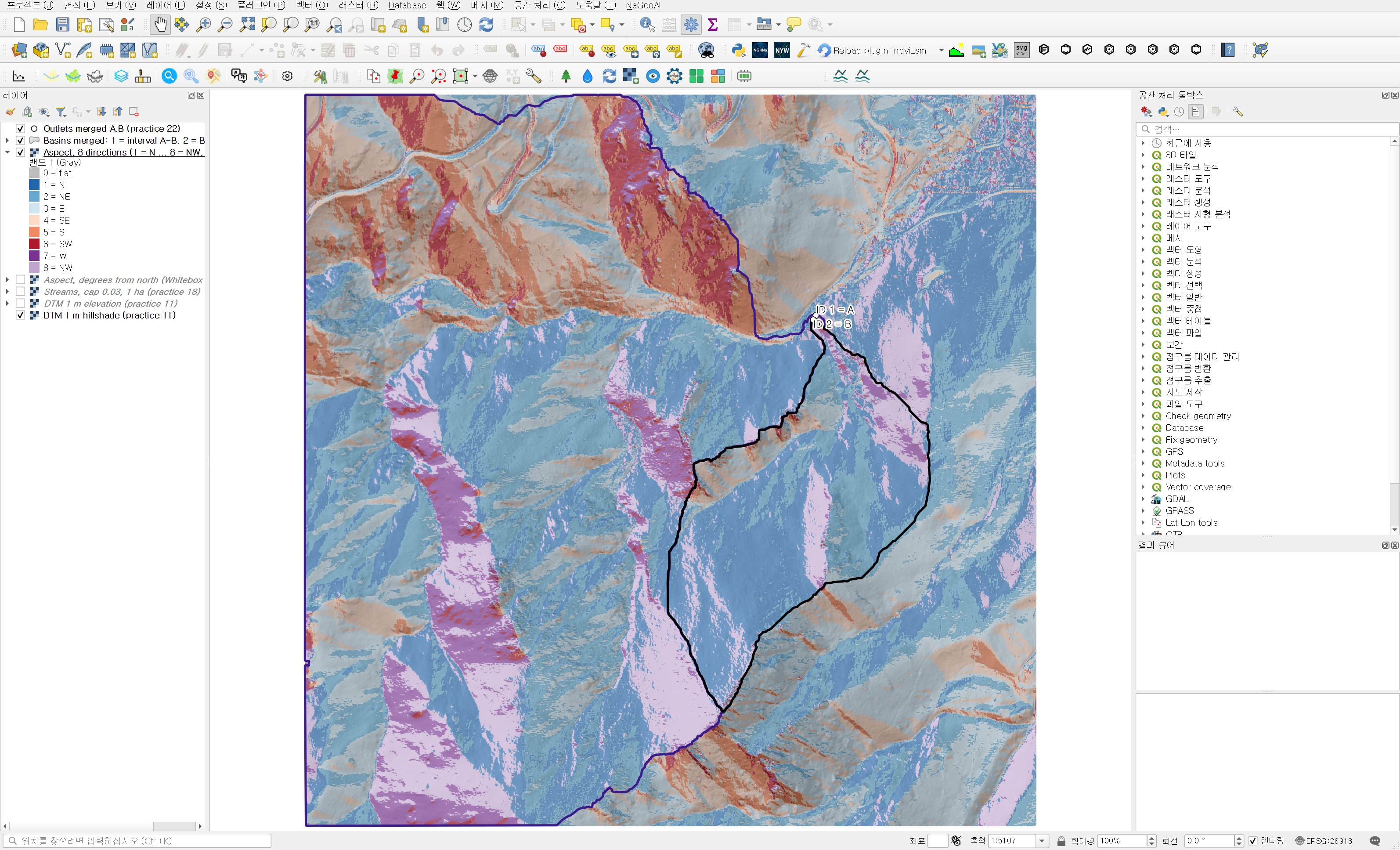
Placed next to Figure 2, the colours are exactly swapped: what was blue is now orange and red, and what was orange is now blue.
Area by direction for each basin
| Field | Value | Reason |
|---|---|---|
| Raster layer | Aspect, 8 directions (1 = N … 8 = NW, 0 = flat) | |
| Band number | Band 1 | |
| Vector layer containing zones | Basins merged: 1 = interval A-B, 2 = B (practice 26) | |
| Output column prefix | h_ | h_0 (flat) to h_8 (NW) |
| Output zones | wb29_basin_aspect_histogram.shp |
| Direction | Interval basin A−B area (m²) | Share | Basin B area (m²) | Share |
|---|---|---|---|---|
| N | 214,252 | 17.58% | 103,300 | 48.87% |
| NE | 267,115 | 21.92% | 41,682 | 19.72% |
| E | 186,782 | 15.33% | 14,445 | 6.83% |
| SE | 152,280 | 12.49% | 8,158 | 3.86% |
| S | 108,260 | 8.88% | 1,616 | 0.76% |
| SW | 59,677 | 4.90% | 870 | 0.41% |
| W | 89,681 | 7.36% | 6,246 | 2.96% |
| NW | 140,732 | 11.55% | 35,055 | 16.59% |
| Flat (code 0) | 1 | 0.00% | 0 | 0% |
| Total | 1,218,780 | 100% | 211,372 | 100% |
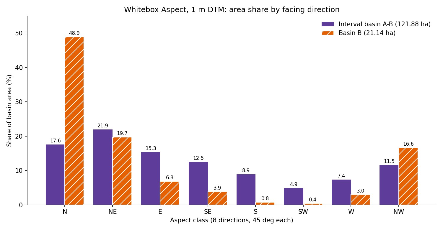
Basin B leans hard to one side. N, NE and NW together make up 85.18%, while SE, S and SW are only 5.04%. It is a narrow valley that rises to the south and drains to a northern outlet, so most of its slopes face north. Averaging aspect as unit vectors gives 8.2° (almost due north), and the mean resultant length (0 for directions spread evenly, 1 for a single direction) is 0.726.
The interval basin is much more even. Its largest sector is NE (21.92%), but E, SE and NW each hold between about 11% and 15%. The three northern sectors total 51.04% against 26.27% for the three southern ones, so north-facing ground still dominates, but the mean resultant length is 0.294, less than half of basin B's. The mean direction is 46.1° (north-east). With several branching valleys inside the larger basin, opposite valley sides appear to cancel each other out.
In session 28 the median slopes of the two basins were nearly the same, around 30°. With aspect, the two basins look quite different. Basin B is almost entirely north-facing, so it has a larger share of shaded slopes even at the same elevation, while the interval basin mixes slopes facing many directions. When comparing basins for insolation, snow or vegetation, this difference may matter more than slope. Here I only checked the distribution; I did not compute insolation.
Independent check
I recomputed the final result with a separate script. Putting the Whitebox aspect values through the same eight-sector rule in numpy left 0 cells different from the QGIS reclassification. Cell counts per sector, from basin polygons rasterised by cell centre, matched the attribute table for every sector in both basins, and the totals matched the session 26 areas.
Against an aspect computed separately with numpy Horn 3×3, over 2,242,171 cells excluding the edges, the median difference was 1.00°, the mean 1.80°, and 99% of cells were within 13.65°. 96.13% of cells fell in the same eight-way sector. The cells with large differences appear to be nearly flat ground, where direction is unstable. On the first run the median of this comparison was 179.0°, so this one check alone is enough to catch a reversed result.
Practical notes
- With WhiteboxTools v2.2.0 Aspect, leave Z Conversion Factor empty. Entering 1.0 produces, without any error, an aspect raster rotated by 180°. I did not test other versions or values other than 1.0.
- Check the aspect result once against terrain you already know, such as the outlet location or stream direction. Just checking that slopes descend toward the valley outlet is enough to catch a reversal.
- North crosses 0°/360°. If the reclassification table does not split it into two rows, only half of the north-facing ground is captured. For averages, use the vector mean rather than the arithmetic mean (the arithmetic mean of 350° and 10° is 180°).
- Flat cells come out as a separate value such as −1. Without a negative range in the reclassification table they can disappear as NoData or mix into north.
- Whitebox aspect refers to the downhill direction. When mixing tools, first align the convention (north 0°, clockwise) and how flat cells are marked.
Next session
After elevation, slope and aspect, the next question is where water gathers. I plan to make a Whitebox topographic wetness index (Wetness Index, TWI) and compare the wetness distribution of the two basins in the same way. The index changes a lot depending on which tools produce the specific contributing area and slope, so I will start with preparing those inputs.
Work notes
This session was run by a QGIS startup script that filled in the same dialogs and ran them, and the screens are captures from that run. The original project was left untouched and the work was done in a copy (QGIS_Play_NaGeoAI_20261118_29_aspect8dir.qgz). The first result, made with Z factor 1.0, was kept separately with try1_zfactor1 in its name, and Figures 1 and 2 are from that run. The direct Whitebox runs and synthetic-plane tests used to find the cause were done separately outside QGIS. The data source is USGS 3DEP (The National Map) tile 13SDE474426, and the original DTM is not redistributed. Figure 6, the shares, the vector means and the independent check come from a separate script that re-reads the output files. QGIS 3.44.15, WhiteboxTools v2.2.0 (wbt_for_qgis plugin). First 12 characters of SHA-256:
- Input DTM 069a9c249240
- Input merged polygons .shp / .dbf 235891ed214a / 67d3965a6d72
- Aspect raster 90bbd5f3c503
- Eight-sector raster 5bd9eb5e5aad
- Zonal histogram .shp / .dbf 235891ed214a / 9173dd77e473
This is an English adaptation of a post in the Korean Whitebox QGIS practice series. The original is here.
This post was drafted with the help of AI tools and reviewed by the author. Tool features and data portals change over time, so check the official documentation when you practice.


Comments
Post a Comment