Whitebox QGIS Practice 31 — Stream Power Index of Two Basins: The Main Channel Set the Mean, the Slopes Set the Median
In practice 30 I compared where two basins are likely to stay wet, using the topographic wetness index (TWI). The same inputs answer the opposite question too. Not where water collects, but where the collected water, running down a slope, has the most power to scour its bed. When I want a first pass over erosion-prone ground before thinking about check dams or drains, the index I reach for is the Stream Power Index (SPI).
The formula is SPI = SCA × tan β. SCA is the D-infinity specific contributing area from practice 30 (m²/m) and β is the slope. TWI is the log of SCA divided by tan β; SPI is SCA multiplied by it. It grows where a cell receives a lot of water from upslope and is steep as well. This time I took the practice 30 outputs as they were, ran Whitebox StreamPowerIndex, and compared the two basins with Zonal statistics. The comparison flipped depending on which summary value I looked at, and most of this post is about that.
Data
I copied the practice 30 inputs and outputs into a new input folder (WB31_Input_20261120). The copies have the same hashes as the originals.
| Input | Origin | Contents |
|---|---|---|
| wb31_input_sca_dinf.tif | Practice 30, DInf Flow Accumulation | D-infinity specific contributing area from the breached DEM of practice 18 (max cost 0.03). 1 m cells, EPSG:26913, 1500×1500 cells |
| wb31_input_slope_deg.tif | Practice 30, Slope | Slope of the same breached DEM in degrees. 0.020° to 88.65°, no 0° cells |
| wb31_input_basins_merged.shp | Practice 26 merged polygons | VALUE 1 = interval basin (A−B) 1,218,780 m², VALUE 2 = basin B 211,372 m² |
| wb31_input_streams_cap0p03.tif | Practice 18 streams | Streams at a 1 ha contributing-area threshold (for the map and for stream-cell statistics) |
The reason for not recomputing SCA and slope is simple. To set practice 30's TWI next to this SPI, both indices have to come from exactly the same SCA and the same slope. Recompute either one and you can no longer tell whether a difference comes from the index or from the inputs.
Step 1: StreamPowerIndex
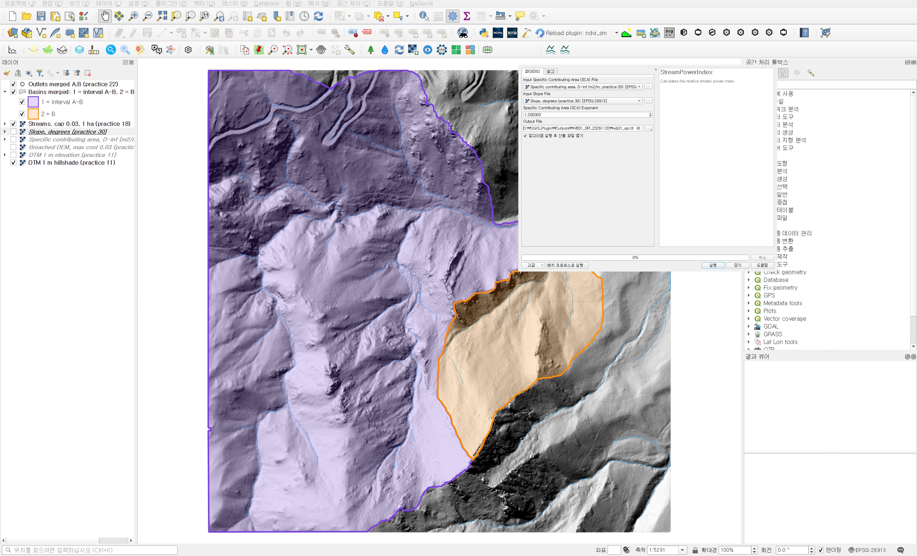
Open Processing Toolbox → WhiteboxTools → Geomorphometric Analysis → StreamPowerIndex. It has three inputs.
| Field | Value | Reason |
|---|---|---|
| Input Specific Contributing Area (SCA) File | Specific contributing area, D-inf (m2/m, practice 30) | It has to be an SCA made with Log-transform turned off. A log-transformed SCA makes the multiplication meaningless. |
| Input Slope File | Slope, degrees (practice 30) | Slope in degrees. The independent check below matched tan taken in degrees. |
| Specific Contributing Area (SCA) Exponent | 1.0 (default) | The p in SPI = SCA^p × tan β. I kept the basic form. It is a research adjustment that weakens or strengthens the area term, and results are only comparable with the same value. |
| Output File | wb31_spi.tif |
The result spans from 0.00044 to 1,719,393, close to ten orders of magnitude. The median is 14.1, but the 99th percentile is 1,469 and the maximum is 1.7 million. The distribution inherits the long tail of SCA, so a linear colour ramp shows a few streams and paints everything else in one colour. I used stepped colours with breaks at 0.1, 1, 10, 100, 1,000 and 10,000. In a QGIS discrete ramp the legend value is the upper end of each class, so navy, for example, means cells above 1,000.
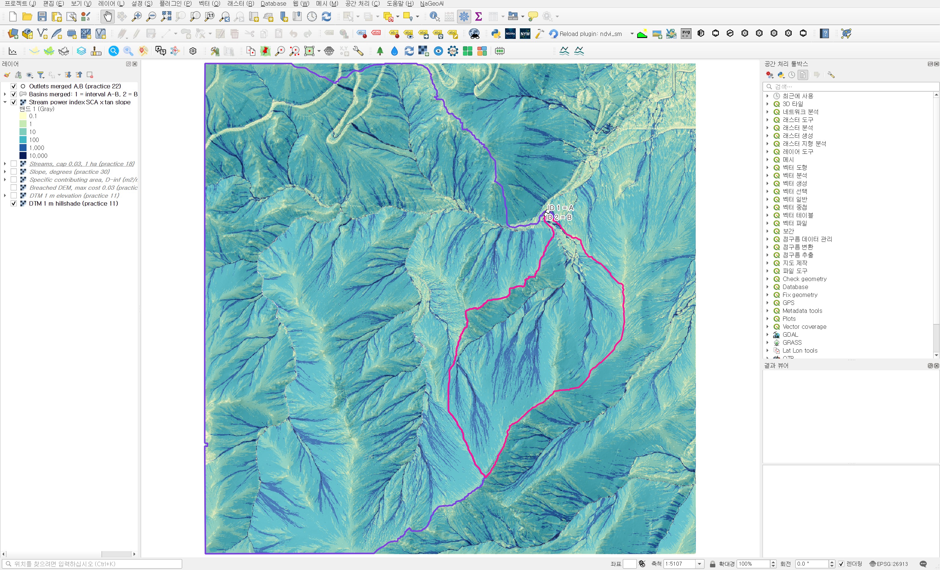
Next to the TWI map (practice 30, figure 4) the valley lines look alike, but they behave differently. TWI is larger on gentle valley floors; along the same line, SPI is larger on the steeper upstream reaches. I zoomed in near the outlets and overlaid the practice 18 streams in red.
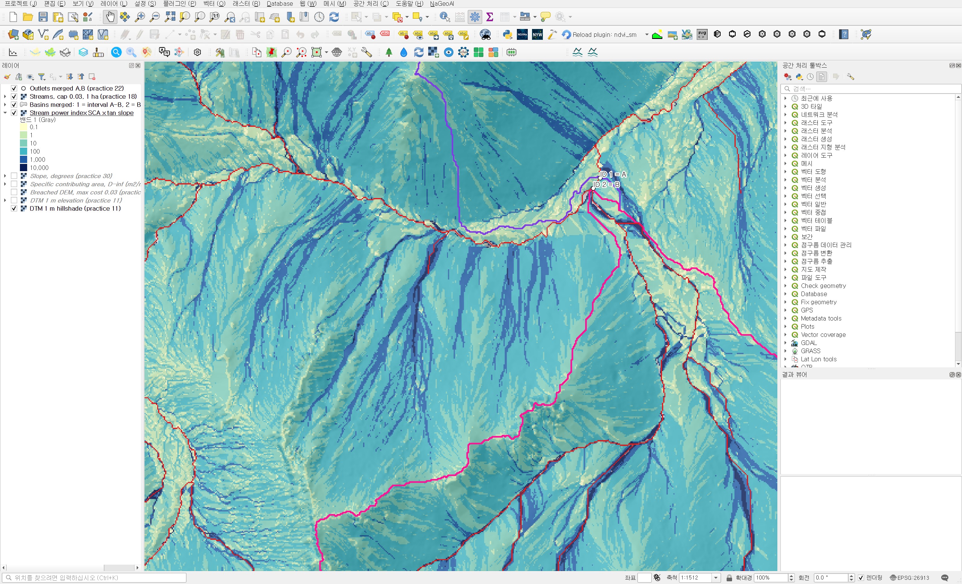
The part worth a second look is the slopes without a red line. Hillslope hollows below the 1 ha stream threshold still carry long navy (above 1,000) and blue (above 100) lines. The contributing area is small, but where the slope is steep the product grows and lands in the same colour class as stream cells. These hollows are exactly where it is easy to say "no channel here, so it is fine" when you only look at extracted streams.
Step 2: Zonal statistics per basin
In Processing Toolbox → Raster analysis → Zonal statistics I used the practice 26 merged polygons and the SPI raster. The prefix is spi_, and the statistics are the same as in practice 30: count, mean, median, standard deviation, minimum and maximum. The output is wb31_basin_spi_stats.shp.
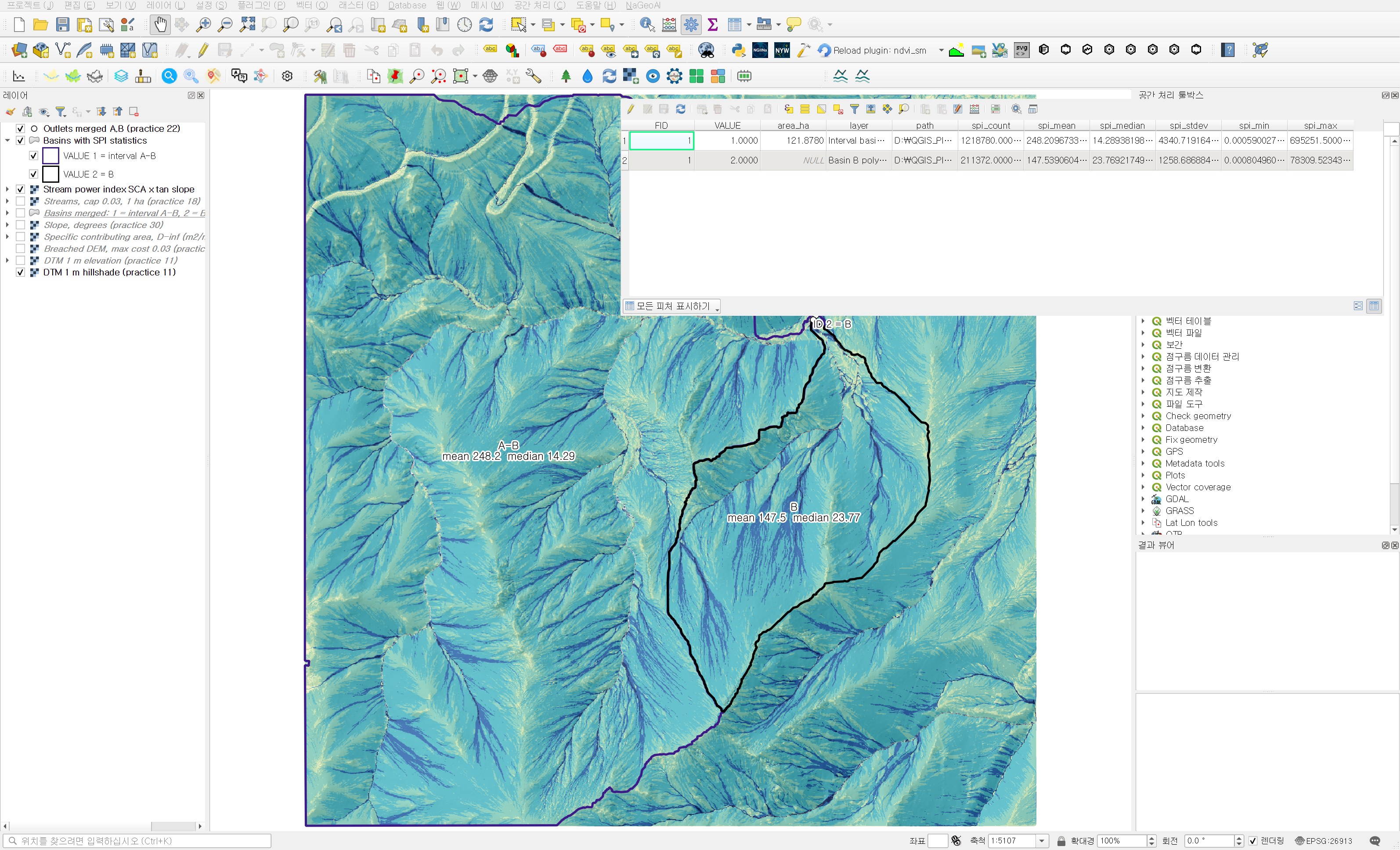
| Item | Interval basin A−B | Basin B |
|---|---|---|
| Cells (m²) | 1,218,780 | 211,372 |
| Mean | 248.2 | 147.5 |
| Median | 14.29 | 23.77 |
| Standard deviation | 4,340.7 | 1,258.7 |
| Maximum | 695,251.5 | 78,309.5 |
| 10th / 90th percentile | 2.24 / 89.97 | 3.50 / 134.08 |
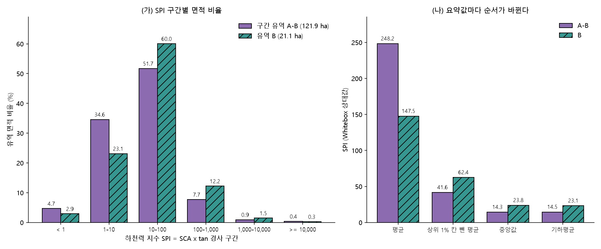
By the mean, the interval basin is 1.7 times basin B. By the median, it is the other way round: B is 1.7 times larger. The standard deviation is 17 times the mean for A−B and 8.5 times for B. With a distribution this skewed, a single mean should not stand for a basin.
Why the mean flipped
I sorted the values and set the top 1% of cells aside.
| Item | Interval basin A−B | Basin B |
|---|---|---|
| Top 1% cells | 12,188 | 2,114 |
| Share of the SPI sum held by the top 1% cells | 83.4% | 58.1% |
| Mean without the top 1% cells | 41.6 | 62.4 |
| Geometric mean | 14.49 | 23.14 |
| Stream cells (1 ha) count / median | 6,390 / 11,493 | 1,371 / 4,895 |
| Median of non-stream cells | 14.17 | 23.52 |
In the interval basin, 1% of the cells hold 83% of the SPI sum. Remove them and the mean drops from 248 to 41.6, below B's 62.4. The main channel of A runs through the interval basin, and its cells have upslope areas in the hundreds of thousands of m², which puts their SPI in the tens or hundreds of thousands. The maximum of 695,252 appears to sit on that main channel. The stream-cell median is also 11,493 in the interval basin, more than twice B's 4,895. In other words, the difference in means was about whether a basin contains the main channel, not about the character of its slopes.
Looking only at non-stream cells, B is 23.5 and the interval basin 14.2. In the class shares of figure 5, B has 12.2% in the 100 to 1,000 class against 7.7% for the interval basin, and 23.1% in the 1 to 10 class against 34.6%. Most of B's slope cells sit one class higher.
Same inputs as TWI, opposite sign
The geometric mean is the back-transformed mean of ln SPI, so it can be split into parts. Since ln SPI = ln SCA + ln tan β, the difference between the basins is:
- Mean ln SCA: B 3.7625, interval basin 3.2619, difference +0.500
- Mean ln tan β: B −0.6208, interval basin −0.5885, difference −0.032
- Sum 0.468, which is a geometric-mean ratio of 23.14 / 14.49 = 1.60
For TWI in practice 30 the same two parts added up as 0.500 + 0.032 = 0.533. TWI divides by tan β, so B's slightly gentler slope raised its TWI; SPI multiplies by it, so the same difference trims SPI a little. The slope term is only about 0.03, though, and most of the difference comes from the 0.5 in ln SCA. On average each slope cell in B receives about e^0.5 ≈ 1.65 times more upslope area, so B is higher in both TWI and SPI. A slope that is both wetter and more erodible sounds contradictory, but both indices look at the same fact, more water passing through, from different angles.
Taken to the field: if the job is managing one main channel, the interval basin comes first. If the concern is scour or sediment from many small hollows on the slopes, I would look at the slopes of basin B first. This reading comes from terrain indices alone and has not been checked against measured erosion or soil conditions.
Independent check
- I recomputed SCA × tan(slope in degrees) with numpy and compared it with the Whitebox output. Over 2,248,166 valid cells the largest relative difference is 6.0×10⁻⁸, and no cell exceeds 10⁻⁵. The exponent of 1.0 and the slope in degrees went in as intended.
- The output SPI is EPSG:26913, 1500×1500, float32, with 1,834 NoData cells (−32768). It shares its grid with the input SCA, slope and DEM, and the NoData count matches the DEM.
- Recomputing the six zonal statistics with basin masks rasterised at cell centres gives differences of 10⁻¹² or less for both basins.
Things to watch in practice
- SPI has an extremely long tail. Comparing basins by the mean alone lets a few main-channel lines decide the result. Report the median, the geometric mean and the share held by the top few percent alongside it.
- Map it with stepped colours on logarithmic breaks. A linear ramp shows only a handful of stream cells.
- SPI is a relative index. Its magnitude depends on DEM resolution, the flow algorithm (D8 or D-infinity) and the SCA exponent p. To compare with another area, rebuild it with the same resolution and settings.
- Look separately at hollows below the stream-extraction threshold. As in figure 3, lines with SPI above 1,000 appear where there is no stream line.
- On a 1 m lidar DEM, man-made features such as road ditches and cut slopes can push SPI up. Check high-value cells against aerial imagery or in the field.
Next session
SPI only measures the relative size of the erosive force. With the same SCA and slope, Whitebox SedimentTransportIndex produces a value corresponding to the slope-length factor (LS) of the soil loss equation (RUSLE). Next time I plan to check whether this SPI and an LS-type index rank the two basins in the same order.
Work notes
This session was run by a QGIS startup script that filled in the same dialogs and ran them, and the screens are captures from that run. The original project was left untouched and the work was done in a copy (QGIS_Play_NaGeoAI_20261120_31_spi.qgz). The data source is USGS 3DEP (The National Map) tile 13SDE474426, and the original DTM is not redistributed. Figure 5, the percentiles, the top 1% share, the geometric means and their split, the stream-cell statistics and the independent check come from a separate script that re-reads the output files. QGIS 3.44.15, WhiteboxTools v2.2.0 (wbt_for_qgis plugin). First 12 characters of SHA-256:
- Input specific contributing area 371c0096063a
- Input slope 0971ac9f4ce6
- Stream power index 17a50232deb2
- Zonal statistics .shp / .dbf 235891ed214a / eb9cdcb01867
This is an English adaptation of a post in the Korean Whitebox QGIS practice series. The original is here.
This post was drafted with the help of AI tools and reviewed by the author. Tool features and data portals change over time, so check the official documentation when you practice.


Comments
Post a Comment