Whitebox QGIS Practice 32 — Sediment Transport Index of Two Basins: A 0.4 Power on Contributing Area Removed the Main-Channel Skew
In practice 31 I compared two basins with the Stream Power Index (SPI). The mean was higher in the interval basin A−B and the median was higher in basin B. What pushed the A−B mean up was the 1% of cells along the main A channel. So what happens if I look at erosion through a different index built from the same inputs? This time I made the Sediment Transport Index (STI) with Whitebox SedimentTransportIndex and compared the same two basins again.
STI is a terrain-based form of the slope-length factor LS in the soil loss equation (USLE/RUSLE). The formula is STI = (n+1) × (SCA / 22.13)n × (sin β / 0.0896)m, and the Whitebox defaults are n = 0.4 and m = 1.3. 22.13 m is the slope length of the standard USLE plot and 0.0896 is the sine of a 9% slope, so the two ratios are dimensionless. The biggest difference from SPI is the 0.4 power on the contributing area. If SCA grows ten thousand times, its part of STI grows only about 40 times.
Data
I copied the practice 31 input folder into a new input folder (WB32_Input_20261121) and added the practice 31 SPI output for comparison. The copies have the same hashes as the originals.
| Input | Origin | Contents |
|---|---|---|
| wb32_input_sca_dinf.tif | Practice 30, DInf Flow Accumulation | D-infinity specific contributing area (m²/m) from the breached DEM of practice 18 (max cost 0.03). 1 m cells, NAD83 UTM 13N EPSG:26913, 1,500×1,500 cells |
| wb32_input_slope_deg.tif | Practice 30, Slope | Slope of the same DEM in degrees |
| wb32_input_spi_wb31.tif | Practice 31, StreamPowerIndex | Stream power index for comparison |
| wb32_input_basins_merged.shp | Practice 26, merged polygons | VALUE 1 = interval basin (A−B) 1,218,780 m², VALUE 2 = basin B 211,372 m² |
| wb32_input_streams_cap0p03.tif | Practice 18, streams | Streams at a 1 ha contributing-area threshold (for the map and stream-cell statistics) |
I reused the practice 30 SCA and slope for the same reason as in practice 31. To compare indices, the inputs have to be identical cell by cell.
Step 1: SedimentTransportIndex
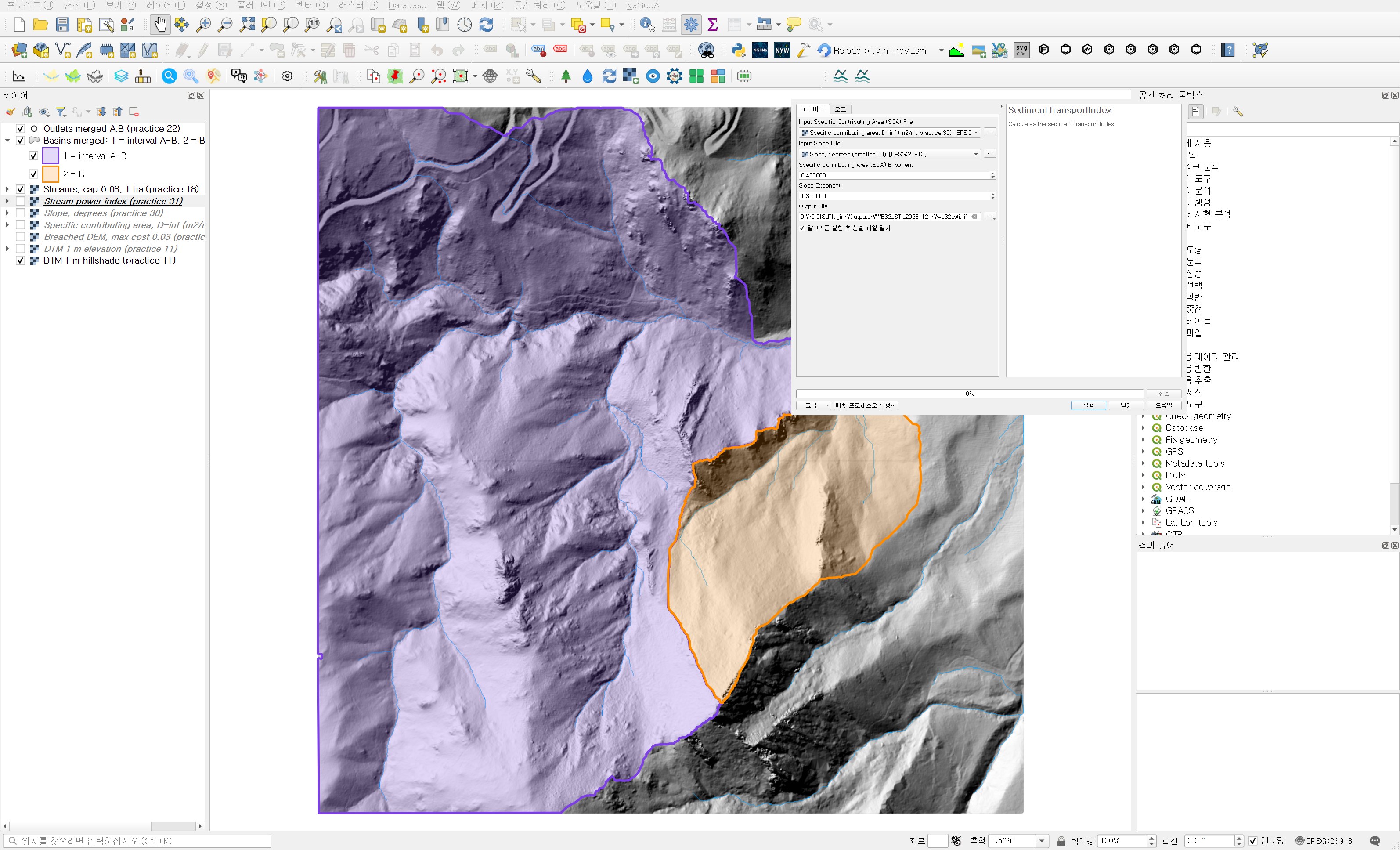
Open Processing Toolbox → WhiteboxTools → Geomorphometric Analysis → SedimentTransportIndex.
| Field | Value | Why |
|---|---|---|
| Input Specific Contributing Area (SCA) File | Specific contributing area, D-inf (m2/m, practice 30) | SCA without log transform. The formula divides it by 22.13 m, so it must be in m²/m. |
| Input Slope File | Slope, degrees (practice 30) | Slope in degrees. The independent check below matched when degrees were converted to radians before taking the sine. |
| Specific Contributing Area (SCA) Exponent | 0.4 (default) | The n in the formula. Values between 0.4 and 0.6 are commonly used. I kept the default for the first comparison. |
| Slope Exponent | 1.3 (default) | The m in the formula. |
| Output File | wb32_sti.tif |
The Whitebox help does not show the formula, so I recomputed it with numpy to see whether the output matches the form above. The form with the (n+1) factor matched within a relative difference of 6×10⁻⁸ over all valid cells. Without the factor every cell would be exactly 1/1.4 of the output, so when comparing with LS from another program, check this factor of 1.4 first.
The value range is already different from practice 31. STI runs from 0.0004 to 1,870, with a median of 12.8 and a 99th percentile of 73.0. SPI spread over nearly ten orders of magnitude up to 1.7 million; the tail is much shorter now. I mapped it with stepped colours at 0.5, 2, 5, 10, 20, 50 and 100. Each legend value is the upper end of its class.
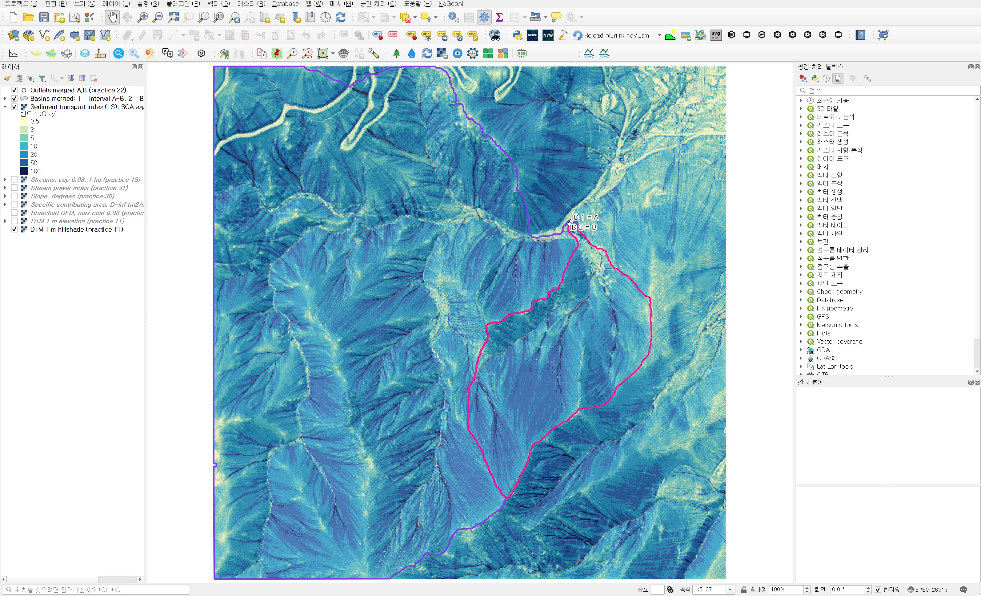
Ranking cells against the practice 31 SPI gives a Spearman rank correlation of 0.908. Broadly the two indices rank the same places high, but the order changes quite a bit. Zooming in near the outlet shows where.
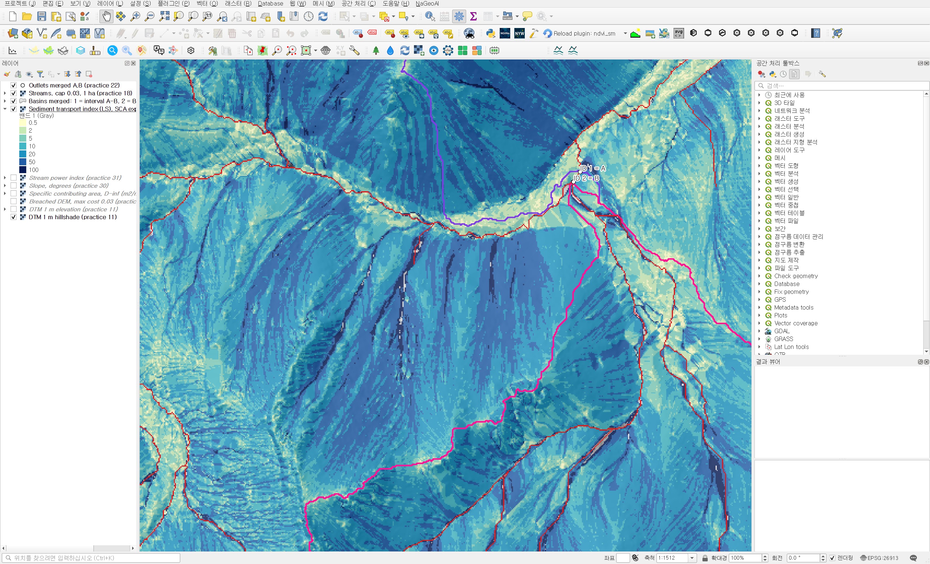
The wide valley floor near the outlet comes out low, in pale yellow and light green. In SPI these main-channel cells were at the very top thanks to their contributing area. In STI the contributing area is pressed down by the 0.4 power and the gentle floor slope is cut further by the 1.3 power, so they drop in rank. Steep slopes and hollows, on the other hand, carry a larger slope term and move up relative to SPI. Across all stream cells the STI median is still higher than on the slopes, 117.6 in the interval basin and 80.1 in B, but it no longer jumps into the thousands and tens of thousands as in practice 31.
Step 2: Zonal statistics per basin
I ran Processing Toolbox → Raster analysis → Zonal statistics with the practice 26 merged polygons and the STI. The prefix is sti_ and the statistics are the same as in practice 31: count, mean, median, standard deviation, minimum and maximum. The output is wb32_basin_sti_stats.shp.
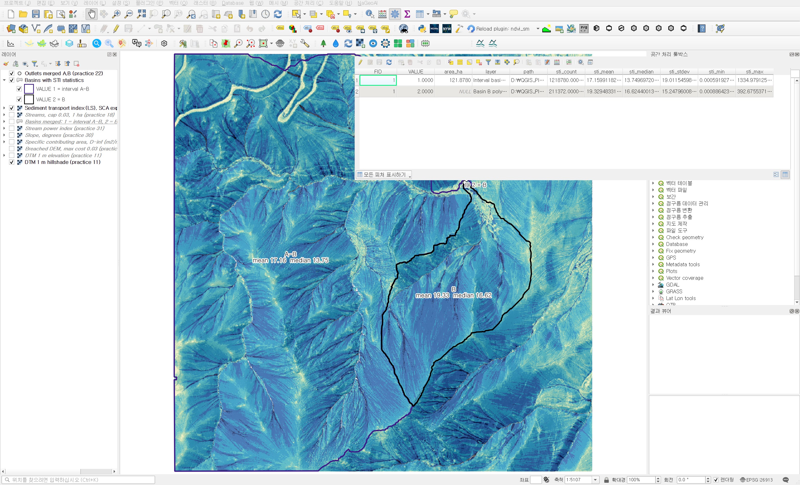
| Item | Interval basin A−B | Basin B |
|---|---|---|
| Cells (m²) | 1,218,780 | 211,372 |
| Mean | 17.16 | 19.33 |
| Median | 13.75 | 16.62 |
| Standard deviation | 19.01 | 15.25 |
| Maximum | 1,335.0 | 392.7 |
| 10th / 90th percentile | 5.38 / 29.49 | 6.20 / 33.49 |
| Geometric mean | 12.82 | 15.15 |
This time B is higher on the mean, the median, the geometric mean and both percentiles. The flip of the mean seen in practice 31 is gone. The standard deviation has also come down to about the size of the mean (for SPI it was 17 and 8.5 times the mean).
Where did the main-channel dominance go?
As in practice 31, I sorted the values and set aside the top 1% of cells.
| Item | Interval basin A−B | Basin B |
|---|---|---|
| Share of the sum held by the top 1% of cells, SPI (practice 31) | 83.4% | 58.1% |
| Share of the sum held by the top 1% of cells, STI | 8.4% | 5.8% |
| STI mean without the top 1% of cells | 15.87 | 18.39 |
| Mean ÷ median, SPI (practice 31) | 17.4 | 6.2 |
| Mean ÷ median, STI | 1.25 | 1.16 |
| Median STI of non-stream cells | 13.70 | 16.55 |
In the interval basin, 1% of cells held 83% of the SPI sum; for STI it is 8.4%. The top 1% holds a little over eight times its share of cells, so the mean stays close to the middle of the distribution. With mean-to-median ratios of 1.25 and 1.16, using the mean as the summary value would not mislead this time.
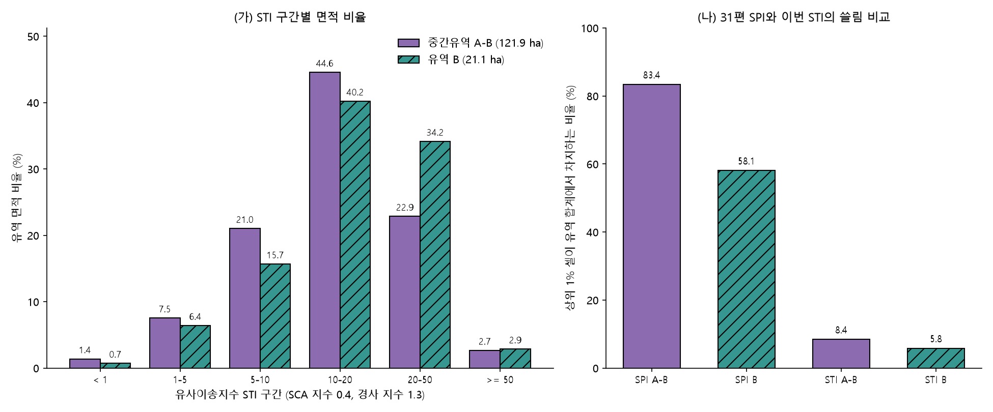
Panel (a) of figure 5 shows that the difference sits in the 20–50 class. In B, 34.2% of the basin area falls there, against 22.9% in the interval basin. The interval basin in turn has more of its area in the 5–10 class, 21.0% against 15.7% in B. The slopes of B as a whole sit one step higher, which is the same picture as the higher SPI median of non-stream cells in B in practice 31.
What lifted B
Since ln STI = ln 1.4 + 0.4(ln SCA − ln 22.13) + 1.3(ln sin β − ln 0.0896), the difference in geometric means splits into an SCA term and a slope term.
- SCA term: 0.4 × (3.7625 − 3.2619) = +0.200
- Slope term: 1.3 × (−0.7853 − (−0.7596)) = −0.034
- Sum 0.167, a geometric-mean ratio of 15.15 / 12.82 ≈ 1.18
The difference of 0.500 in mean ln SCA is the same value as in practices 30 and 31. What changed is the coefficient in front of it. In SPI it was multiplied by 1 and entered as 0.500; in STI it is multiplied by 0.4 and shrinks to 0.200. The mean slopes of the two basins are almost the same, 30.3° and 29.5°, so the slope term is small again and the 1.3 power trims B slightly. In the end B leads for the same reason as in practice 31: its slope cells receive more area from upslope on average. That effect is smaller now, but the extreme main-channel values are pressed down with it, so the mean finally shows the difference as it is.
In field terms, the interpretation from practice 31 settles on one side. For hillslope erosion and sediment delivery, B is the place to look first. Bed scour in the main channel is a question for SPI or hydraulic calculations, not STI. This is again a reading from terrain indices alone, not something checked against measured soil loss.
Independent check
- I recomputed 1.4 × (SCA/22.13)0.4 × (sin β/0.0896)1.3 with numpy and compared it with the Whitebox output. Over 2,248,166 valid cells the maximum absolute difference was 5.1×10⁻⁵, the maximum relative difference 6.0×10⁻⁸, and no cell exceeded 10⁻⁵.
- The STI output is EPSG:26913, 1,500×1,500 cells, float32, NoData −32768 in 1,834 cells. Its grid matches the input SCA, slope, SPI and DEM, and the NoData count matches the DEM. No cell has a value of 0.
- Recomputing the six zonal statistics with basin masks rasterised at cell centres gave differences of 10⁻¹³ or less in both basins.
Practical points
- STI corresponds to the LS factor; it is not soil loss. To get soil loss you multiply by the rainfall (R), soil (K), cover (C) and support practice (P) factors. The basin comparison here assumes those factors are equal.
- The USLE family is meant for sheet and rill erosion on hillslopes. STI on stream cells does not describe bed scour, so it is better to exclude stream cells from basin summaries or look at them separately.
- The standard USLE plot has a 9% slope, while the mean slope of these basins is around 30°. These slopes are far outside the plot conditions, so use the values as relative ranks within the area rather than as absolute numbers.
- When comparing with LS from another tool, first align the (n+1) factor, the exponents n and m, the slope unit (degrees or percent) and the SCA unit (m²/m or cell count). A single mismatch changes the values several-fold.
- SPI and STI answer different questions from the same inputs. SPI shows whether force concentrates in one main channel; STI shows erosion potential across the slopes. Checking whether both indices rank the basins the same way makes the interpretation more solid.
Next session
This comparison comes from a single combination, n = 0.4 and m = 1.3. Next time I plan to check whether B still leads with other combinations, such as n raised to 0.6 or a different m, and how sensitive the rank correlation and the basin order are to the exponents.
Work notes
This session was run by a QGIS startup script that filled in the same dialogs and ran them, and the screens are captures from that run. The original project was left untouched and the work was done in a copy (QGIS_Play_NaGeoAI_20261121_32_sti.qgz). The data source is USGS 3DEP (The National Map) tile 13SDE474426, and the original DTM is not redistributed. Figure 5, the percentiles, the top 1% share, the geometric means and their split, the stream-cell statistics, the rank correlation and the independent check come from a separate script that re-reads the output files. QGIS 3.44.15, WhiteboxTools v2.2.0 (wbt_for_qgis plugin). First 12 characters of SHA-256:
- Input specific contributing area 371c0096063a
- Input slope 0971ac9f4ce6
- Sediment transport index d2bdec73e68e
- Zonal statistics .shp / .dbf 235891ed214a / 3a4a3aaafb30
This is an English adaptation of a post in the Korean Whitebox QGIS practice series. The original is here.
This post was drafted with the help of AI tools and reviewed by the author. Tool features and data portals change over time, so check the official documentation when you practice.


Comments
Post a Comment